Bayesian Support Vector Regression Using a Unified Loss function
[email protected]
Wei Chu S. Sathiya Keerthi∗
[email protected] [email protected]
Chong Jin Ong
Control Division, Department of Mechanical Engineering, National University of Singapore, 10 Kent Ridge Crescent, Singapore, 119260
Abstract In this paper, we employ a unified loss function, called the soft insensitive loss function, for Bayesian support vector regression. We follow standard Gaussian processes for regression to set up the Bayesian framework, in which the unified loss function is attempted in likelihood evaluation. Under this framework, the maximum a posteriori estimate on the function values corresponds to the solution of an extended support vector regression problem. Bayesian methods are used to implement model adaptation, while keeping the merits of support vector regression, such as quadratic programming and sparseness. Moreover, we put forward error bar in making predictions. Experimental results on simulated and real-world data sets indicate that the approach works well even on large data sets. 1. Introduction The application of Bayesian techniques to neural networks was pioneered by Buntine and Weigend (1991), MacKay (1992) and Neal (1992). These works are reviewed in Bishop (1995), MacKay (1995) and Lampinen and Vehtari (2001). Unlike standard neural network design, the Bayesian approach considers probability distributions in the weight space of the network. Together with the observed data, prior distributions are converted to posterior distributions through the use of Bayes’ theorem. Neal (1996) observed that a Gaussian prior for the weights approaches a Gaussian process for functions as the number of hidden units approaches infinity. Inspired by Neal’s work, Williams and Rasmussen (1996) extended the use of Gaussian process prior to higher dimensional regression problems that have been traditionally tackled with other techniques, such as neural networks, decision trees etc, and good results have been obtained. Regression with Gaussian processes (GPR) is reviewed in Williams (1998). The important advantage of GPR models over other non-Bayesian models is the explicit probabilistic formulation. This not only builds the ability to infer hyperparameters in Bayesian framework but also provides confidence intervals in prediction. The drawback of GPR models lies in the huge computational cost for large sets of data. Support vector machines (SVM) for regression (SVR), as described by Vapnik (1995), exploit the idea of mapping input data into a high dimensional (often infinite) reproducing kernel ∗
All the correspondences should be addressed to S. Sathiya Keerthi.
1
Hilbert space (RKHS) where a linear regression is performed. The advantages of SVR are: a global minimum solution as the minimization of a convex programming problem; relatively fast training speed; and sparseness in solution representation. The performance of SVR crucially depends on the shape of the kernel function and other hyperparameters that represent the characteristics of the noise distribution in the training data. Re-sampling approaches, such as cross-validation (Wahba, 1990), are commonly used in practice to decide values of these hyperparameters, but such approaches are very expensive when a large number of parameters are involved. Typically, Bayesian methods are regarded as suitable tools to determine the values of these hyperparameters. There is some literature on Bayesian interpretations of SVM. For classification, Kwok (2000) built up MacKay’s evidence framework (MacKay, 1992) using a weight-space interpretation. Seeger (1999) presented a variational Bayesian method for model selection, and Sollich (2002) proposed Bayesian methods with normalized evidence and error bar. In SVM for regression (SVR), Law and Kwok (2001) applied MacKay’s Bayesian framework to SVR in the weight space. Gao et al. (2002) derived the evidence and error bar approximation for SVR along the way proposed by Sollich (2002). In these two approaches, the lack of smoothness of the ǫ-insensitive loss function (ǫ-ILF) in SVR may cause inaccuracy in evidence evaluation and inference. To improve the performance of Bayesian inference, we employ a unified non-quadratic loss function for SVR, called the soft insensitive loss function (SILF). The SILF is C 1 smooth. Further, it possesses the main advantages of ǫ-ILF, such as insensitivity to outliers and sparseness in solution representation. We follow standard GPR to set up Bayesian framework, and then employ SILF in likelihood evaluation. Maximum a posteriori (MAP) estimate of the function values results in an extended SVR problem, so that quadratic programming can be employed to find the solution. Optimal hyperparameters can then be inferred by Bayesian techniques with the benefit of sparseness, and error bar can also be provided in making predictions. The paper is organized as follows: in section 2 we review the standard framework of regression with Gaussian processes; in section 3 we propose SILF as a unified non-quadratic loss functions, and describe some of its useful properties; in section 4 we employ the SILF as loss function in the MAP estimate of these function values, and then formulate the consequent optimization problem as a convex quadratic programming problem; hyperparameter inference is discussed in section 5 and predictive distribution is discussed in section 6; we show the results of numerical experiments that verify the approach in section 7 and we conclude in section 8. 2. Bayesian Framework in Gaussian Processes In regression problems, we are given a set of training data D = {(xi , yi )|i = 1, . . . , n, xi ∈ Rd , yi ∈ R} which is collected by randomly sampling a function f , defined on Rd . As the measurements are usually corrupted by additive noise, training samples can be represented as yi = f (xi ) + δi
i = 1, 2, . . . , n
(1)
where the δi are independent, identically distributed (i.i.d.) random variables, whose distributions are usually unknown. Regression aims to infer the function f , or an estimate of it, from the finite data set D. In the Bayesian approach, we regard the function f as the realization of a random field with a known prior probability. The posterior probability of f given the training data D can then be derived by Bayes’ theorem: P(f |D) =
P(D|f )P(f ) P(D) 2
(2)
where f = [f (x1 ), f (x2 ), . . . , f (xn )]T , P(f ) is the prior probability of the random field and P(D|f ) is the conditional probability of the data D given the function values f which is exactly Qn i=1 P(yi |f (xi )). Now we follow the standard Gaussian processes (Williams and Rasmussen, 1996; Williams, 1998) to describe a Bayesian framework. 2.1 Prior Probability We assume that the collection of training data is the realization of random variables f (xi ) in a zero mean stationary Gaussian process indexed by xi . The Gaussian process is specified by the covariance matrix for the set of variables {f (xi )}. The covariance between the outputs corresponding to inputs xi and xj could be defined as à ! d κX l l 2 Cov[f (xi ), f (xj )] = Cov(xi , xj ) = κ0 exp − (x − xj ) + κb (3) 2 l=1 i where κ > 0, κ0 > 0 denotes the average power of f (x), κb > 0 denotes the variance of the offset to the function f (x), and xl denotes the l-th element of the input vector x. Such a covariance function expresses the idea that cases with nearby inputs have highly correlated outputs. Note that the first term in (3) is the Gaussian kernel in SVM, while the second term corresponds to the variance of the bias in classical SVR (Vapnik, 1995). Other kernel functions in SVM, such as polynomial kernel, spline kernel (Wahba, 1990), ANOVA decomposition kernel (Saunders et al., 1998) etc., or their combinations can also be used in covariance function, but we only focus on Gaussian kernel in the present work. Thus, the prior probability of the functions is a multivariate Gaussian with zero mean and covariance matrix as follows µ ¶ 1 1 T −1 P(f ) = exp − f Σ f (4) Zf 2 p where f = [f (x1 ), f (x2 ), . . . , f (xn )]T , Zf = (2π)n/2 |Σ| and Σ is the n × n covariance matrix whose ij-th elements is Cov[f (xi ), f (xj )].1 2.2 Likelihood Function The probability P(D|f ), known as likelihood, is essentially a model of the noise. If the additive noise δi in (1) is i.i.d. with probability distribution P(δi ), P(D|f ) can be evaluated by: P(D|f ) =
n Y i=1
P(yi − f (xi )) =
n Y i=1
P(δi )
(5)
Furthermore, P(δi ) is often assumed to be of the exponential form such that P(δi ) ∝ exp(C · ℓ(δi )) where ℓ(·) is called the loss function and C is a parameter greater than zero. Thus, the likelihood function can also be expressed as à ! n X P(D|f ) ∝ exp C · ℓ(yi − f (xi )) (6) i=1
1 If the covariance is defined using (3), Σ is symmetric and positive definite if {xi } is a set of distinct points in Rd (Micchelli, 1986).
3
Hence, the loss function characterizes the noise distribution, which together with the prior probability P(f ), determines the posterior probability P(D|f ). 2.3 Posterior Probability Based on Bayes’ theorem (2), prior probability (4) and the likelihood (5), the posterior probability of f can be written as 1 (7) P(f |D) = exp (−S(f )) Z R P where S(f ) = C ni=1 ℓ (yi − f (xi )) + 12 f T Σ−1 f and Z = exp(−S(f ))df . The maximum a posteriori (MAP) estimate of the function values is therefore the minimizer of the following optimization problem:2 n X 1 min S(f ) = C (8) ℓ (yi − f (xi )) + f T Σ−1 f f 2 i=1 Let f MP be the optimal solution of (8). If the loss function we used in (8) is differentiable, the derivative of S(f ) with respect to f should be zero at f MP , i.e. ¯ ¯ n X ∂S(f ) ¯¯ ∂ℓ (yi − f (xi )) ¯¯ + Σ−1 f = 0 =C ¯ ¯ ∂f ¯f MP ∂f i=1 f MP ¯ ∂ℓ(yi −f (xi )) ¯ ∀i, and w as the Let us define the following set of unknowns wi = − C ∂f (xi ) ¯ f (xi )=fMP (xi )
column vector containing {wi }. Then f MP can be written as: f MP = Σ · w
(9)
The elegant form of a minimizer of (8) is also known as the representer theorem (Kimeldorf and Wahba, 1971). A generalized representer theorem can be found in Sch¨olkopf et al. (2001), in which the loss function is merely required as any strictly monotonically increasing function ℓ : R → [0, +∞). We can further decompose the solution (9) into the form n n n X X X wi · K(x, xi ) + b wi = κ0 f MP (x) = wi · κ0 · K(x, xi ) + κb i=1
i=1
(10)
i=1
³ ´ P where b = κb i=1 wi and K(x, xi ) = exp − κ2 dl=1 (xl − xli )2 is just the Gaussian kernel in classical SVR, to show the significance of the hyperparameter in regression function. The contribution of each pattern to the regression function depends on its wi in (10), and κ0 is the average power of all the P training patterns. κb only involves in the bias term b in (10) that might be trivial if the sum ni=1 wi is very small. Pn
2.4 Hyperparameter Evidence
The Bayesian framework we described is conditional on the parameters in the prior distribution and the parameters in likelihood function, which can be collected, as θ, the hyperparameter vector. The normalizing constant P(D) in (2), more exactly P(D|θ), is irrelevant to the inference of the functions f , but it becomes important in hyperparameter inference, and it is known as the evidence of the hyperparameters θ (MacKay, 1992). 2 S(f ) is a regularized functional. As for the connection to regularization theory, Evgeniou et al. (1999) have given a comprehensive discussion.
4
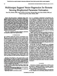
3. A Unified Non-quadratic Loss Function There are several choices for the form of the loss function. In standard Gaussian processes for regression (GPR), Gaussian noise model is used in likelihood function (Williams and Rasmussen, 1996; Williams, 1998), which is of the form ¶ µ 1 δ2 PG (δ) = √ exp − 2 . 2σ 2πσ where the parameter σ 2 is the noise variance and the loss function is the quadratic function ℓ(δ) = 12 δ 2 . The Gaussian process prior for the functions f is conjugated with the Gaussian likelihood to yield a posterior distribution over functions that can be used in hyperparameter inference and prediction. The posterior probability over functions can be carried out exactly using matrix operations in the GPR formulation. This is one of the reasons that the Gaussian noise model is popularly used. However, one of the potential difficulties of the quadratic loss function is that it receives large contributions from outliers. If there are long tails on the noise distributions then the solution can be dominated by a very small number of outliers, which is an undesirable result. Techniques that attempt to solve this problem are referred to as robust statistics (Huber, 1981). Nonquadratic loss functions have been introduced to reduce the sensitivity to the outliers. The three non-quadratic loss functions commonly used in regression problems are: 1. the Laplacian loss function defined as ℓ(δ) = |δ|; 2. the Huber’s loss function (Huber, 1981) defined as δ2 if |δ| ≤ 2ǫ ℓ(δ) = 4ǫ |δ| − ǫ otherwise. where ǫ > 0;
3. the e-insensitive loss function (ǫ-ILF) (Vapnik, 1995), ½ 0 if |δ| ≤ ǫ ℓ(δ) = |δ| − ǫ otherwise. where ǫ > 0. From their definitions and Figure 1, we notice that Huber’s loss function and ǫ-ILF approach the Laplacian loss function as ǫ → 0. In addition, Laplacian loss function and ǫ-ILF are nonsmooth, while Huber’s loss function is a C 1 smooth function which can be thought of as a mixture between Gaussian and Laplacian loss function. ǫ-ILF is special in that it gives identical zero penalty to small noise values. Because of this, training samples with small noise that fall in this flat zero region are not involved in the representation of regression functions, as known in SVR. This simplification of computational burden is usually referred to as the sparseness property. All the other loss functions mentioned above do not enjoy this property since they contribute a positive penalty to all noise values other than zero. On the other hand, quadratic and Huber’s loss function are attractive because they are 5
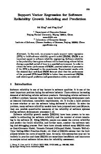
differentiable, a property that allows appropriate approximations to be used in the Bayesian approach. Based on these observations, we blend their desirable features together and introduce a novel loss function, namely soft insensitive loss function. The soft insensitive loss function (SILF) can be seen as a unified version of the above-mentioned non-quadratic loss functions. It is defined as: ¡ ¢ −δ − ǫ if δ ∈ ∆C ∗ = − ∞, −(1 + β)ǫ (δ + (1 − β)ǫ)2 if δ ∈ ∆M ∗ = [−(1 + β)ǫ, −(1 − β)ǫ] 4βǫ 0 if δ ∈ ∆0 = (−(1 − β)ǫ, (1 − β)ǫ) ℓǫ,β (δ) = (11) 2 (δ − (1 − β)ǫ) if δ ∈ ∆M = [(1 − β)ǫ, (1 + β)ǫ] 4βǫ ¡ ¢ δ−ǫ if δ ∈ ∆C = (1 + β)ǫ, +∞
where 0 < β ≤ 1 and ǫ > 0. There is a profile of SILF as shown in Figure 2. The properties of SILF are entirely controlled by two parameters, β and ǫ. For a fixed ǫ, SILF approaches the ǫ-ILF as β → 0; on the other hand, as β → 1, it approaches the Huber’s loss function. In addition, SILF becomes the Laplacian loss function as ǫ → 0. Held ǫ at some large value and let β → 1, the SILF approach the quadratic loss function for all practical purposes. The derivatives of the loss function are needed in Bayesian methods. The first order derivative of SILF can be written as −1 if δ ∈ ∆C ∗ δ + (1 − β)ǫ if δ ∈ ∆M ∗ 2βǫ dℓǫ,β (δ) 0 if δ ∈ ∆0 = dδ δ − (1 − β)ǫ if δ ∈ ∆M 2βǫ 1 if δ ∈ ∆C
where 0 < β ≤ 1 and ǫ > 0. The loss function is not twice continuously differentiable, but the second order derivative exists almost everywhere: 1 2 d ℓǫ,β (δ) if δ ∈ ∆M ∗ ∪ ∆M (12) = 2βǫ 2 0 otherwise dδ
where 0 < β ≤ 1 and ǫ > 0.
We now derive some of the properties of the noise model corresponding to SILF, as they are useful in the subsequent development. The density function of the additive noise in measurement corresponding to the choice of SILF is PS (δ) = 1 where = ZS
Z
¡ ¢ 1 exp − C · ℓǫ,β (δ) ZS
(13)
¡ ¢ exp − C · ℓǫ,β (δ) dδ. It is possible to evaluate the integral and write ZS as: r
ZS = 2(1 − β)ǫ + 2
³p ´ 2 ¡ ¢ πβǫ · erf Cβǫ + exp − Cβǫ C C 6
(14)
Z z 2 where erf(z) = √ exp(−t2 ) dt. The mean of the noise is zero, and the variance of the noise π 0 σn2 can be written as: r µ ½ ¶ ´ ³p 3 3 πβǫ 2βǫ (1 − β) ǫ 2 2 2 2 Cβǫ + + (1 − β) ǫ erf σn = ZS 3 C ¶ ¾ µ 2 C (15) 2 4(1 − β)βǫ2 ǫ (1 − β)2 2ǫ(1 + β) + + + 3 exp(−Cβǫ) + C C C2 C Remark 1 We now give an interpretation for SILF, which is an extension of that given by Pontil et al. (1998) for ǫ-ILF. If we discard the popular assumption that the distribution of the noise variables δi is a zero-mean Gaussian, but assume that the noise variables δi have a Gaussian distribution P(δi |σi , ti ) having its own standard deviation σi and its mean ti that are i.i.d. random variables with density functions µ(σi ) and λ(ti ) respectively. Then we can compute the marginal of the noise probability by integrating over σi and ti as follows: Z Z P(δi ) = dσi dti P(δi |σi , ti )λ(ti )µ(σi ) (16) The probability (16) can also be evaluated in the form of loss function as (13). Under such settings, it is possible (Chu et al., 2001) to find a Rayleigh distribution on σi and a specific distribution on ti , such that the evaluations of expression (13) and (16) are equivalent. Therefore, the use of SILF can also be explained as a general Gaussian noise model with the specific distribution on the mean and the standard deviation. 4. Support Vector Regression We now describe the optimization problem (8) arising from the introduction of SILF (13) as the loss function. In this case, the MAP estimate of the function values is the minimizer of the following problem n X 1 min S(f ) = C ℓǫ,β (yi − f (xi )) + f T Σ−1 f (17) f 2 i=1 As usual, by introducing two slack variables ξi and ξi∗ , (17) can be restated as the following equivalent optimization problem, which we refer to as the primal problem: ∗
min∗ S(f , ξ, ξ ) = C
f,ξ,ξ
n X i=1
1 ℓǫ,β (ψ(ξi ) + ψ(ξi∗ )) + f T Σ−1 f 2
(18)
subject to
where
yi − f (xi ) ≤ (1 − β)ǫ + ξi f (xi ) − yi ≤ (1 − β)ǫ + ξi∗ ξi ≥ 0, ξi∗ ≥ 0 ∀i ψ(π) =
½
π2 4βǫ
if π ∈ [0, 2βǫ) π − βǫ if π ∈ [2βǫ, +∞)
(19)
(20)
Standard Lagrangian techniques (Fletcher, 1987) are used to derive the dual problem. Let αi ≥ 0, αi∗ ≥ 0, γi ≥ 0 and γi ≥ 0 ∀i be the corresponding Lagrange multipliers for the 7
inequality in (19). The Lagrangian for the primal problem is: n n X X 1 γi ξi − γi∗ ξi∗ ℓǫ,β (ψ(ξi ) + ψ(ξi∗ )) + f T Σ−1 f − 2 i=1 i=1 i=1 n n X X − αi (ξi + (1 − β)ǫ − yi + f (xi )) − αi∗ (ξi∗ + (1 − β)ǫ + yi − f (xi ))
L(f , ξ, ξ ∗ ; α, α∗ , ξ, ξ ∗ ) = C
n X
i=1
(21)
i=1
The KKT conditions for the primal problem require f (xi ) =
n X j=1
(αj − αj∗ )Cov(xi , xj )
∂ψ(ξi ) = αi + γi ∂ξi ∂ψ(ξi∗ ) = αi∗ + γi∗ C ∂ξi∗ C
∀i
(22)
∀i
(23)
∀i
(24)
Based on the definition of ψ(·) given by (20) and the constraint conditions (23) and (24), the equality constraint on Lagrange multipliers can be explicitly written as αi + γi = C
ξi for 0 ≤ ξi < 2βǫ and αi + γi = C for ξi ≥ 2βǫ 2βǫ
∀i
(25)
ξi∗ for 0 ≤ ξi∗ < 2βǫ and αi∗ + γi∗ = C for ξi∗ ≥ 2βǫ ∀i (26) + =C 2βǫ If we collect all terms involving ξi in the Lagrangian (21), we get Ti = Cψ(ξi ) − (αi + γi )ξ. Using (20) and (25) we can rewrite Ti as (αi + γi )2 βǫ − if 0 ≤ αi + γi < C Ti = (27) C −Cβǫ if αi + γi = C αi∗
γi∗
2
Thus ξi can be eliminated if we set Ti = − (αi +γCi ) βǫ and introduce the additional constraints, 0 ≤ αi + γi ≤ C. The same arguments can be repeated for ξi∗ . Then the dual problem becomes a maximization problem involving only the dual variables α, α∗ , γ and γ ∗ : n n n X 1 XX (αi − αi∗ )(αj − αj∗ )Cov(xi , xj ) + (αi − αi∗ )yi 2 i=1 j=1 i=1 n n X X ¡ ¢ βǫ (αi + γi )2 + (αi∗ + γi∗ )2 − (αi + αi∗ )(1 − β)ǫ − C i=1 i=1
max S(α, α∗ , γ, γ ∗ ) = − ∗ ∗
α,α ,γ,γ
(28)
subject to αi ≥ 0, γi ≥ 0, αi∗ ≥ 0, γi∗ ≥ 0, 0 ≤ αi + γi ≤ C and 0 ≤ αi∗ + γi∗ ≤ C, ∀i. As the last term in (28) is the only one where γi and γi∗ appear, (28) is maximal when γi = 0 and γi∗ = 0 ∀i. Therefore, the dual problem can be finally simplified as n n n X 1 XX ∗ ∗ (αi − αi )(αj − αj )Cov(xi , xj ) − min S(α, α ) = (αi − αi∗ )yi α,α∗ 2 i=1 j=1 i=1 n n X X ¢ ¡ 2 βǫ αi + αi∗ 2 + (αi + αi∗ )(1 − β)ǫ + C i=1 i=1 ∗
8
(29)
subject to 0 ≤ αi ≤ C and 0 ≤ αi∗ ≤ C.
Obviously, the dual problem (29) is a convex quadratic programming problem. Matrix-based quadratic programming techniques that use the “chunking” idea can be employed (Vanderbei, 2001). Popular SMO algorithms for classical SVR (Smola and Sch¨olkopf, 1998; Shevade et al., 2000) could also be adapted for its solutions. For more details about the adaptation, refer to Appendix A. The optimal value of the primal variables f can be obtained from the solution of (29) as f MP = Σ · (α − α∗ )
(30)
where α = [α1 , α2 , . . . , αn ]T and α∗ = [α1∗ , α2∗ , . . . , αn∗ ]T . This expression, which is consistent with (9), is the solution to MAP estimate of the function values f MP in the Gaussian processes.3 At the optimal solution, the training samples (xi , yi ) with associated αi − αi∗ satisfying 0 < |αi − αi∗ | < C are usually called off-bound support vectors (SVs); the samples with |αi − αi∗ | = C are on-bound SVs, and the samples with |αi − αi∗ | = 0 are non-SVs. From the definition of SILF (11) and the equality constraints (25) and (26), we notice that the noise δi in (1) associated with on-bound SVs should belong to ∆C ∗ ∪ ∆C , while δi associated with off-bound SVs should belong to the region ∆M ∗ ∪ ∆M .4 Remark 2 From (12), the second derivative of ℓǫ,β (δi ) is not continuous at the boundary of ∆M ∗ ∪ ∆M . The lack of C 2 continuity may have impact on the evaluation of the evidence P(D|θ) (to be discussed later in Section 5). However, it should be pointed out that the noise δi seldom falls on the boundary of ∆M ∗ ∪ ∆M exactly, since it is of low probability for a continuous random variable to be realized on some particular values. 4.1 General Formulation Like SILF, the dual problem in (29) is a generalization of several SVR formulations. More exactly, when β = 0 (29) becomes the SVR formulation using ǫ-ILF; when β = 1, (29) becomes that when the Huber’s loss function is used; and when β = 0 and ǫ = 0, (29) becomes that for the case of the Laplacian loss function. Moreover, for the case of Gaussian noise model (3), the dual problem becomes min∗
α,α
n n n n X ¢ 1 XX σ2 X ¡ 2 αi + αi∗ 2 (αi − αi∗ )(αj − αj∗ )Cov(xi , xj ) − (αi − αi∗ )yi + 2 i=1 j=1 2 i=1 i=1
(31)
subject to αi ≥ 0 and αi∗ ≥ 0 ∀i, where σ 2 is the variance of the additive Gaussian noise. The optimization problem (29) is equivalent to the general SVR (29) with β = 1 and 2ǫ/C = σ 2 provided that we keep upper bound C large enough to prevent any αi and αi∗ from reaching the upper bound at the optimal solution. If we take the implicit constraint αi · αi∗ = 0 into account and then denote αi − αi∗ as νi , it is found that the formulation (31) is actually a much simpler case as n n n n X 1 XX σ2 X 2 min ν (32) νi νj Cov(xi , xj ) − νi y i + ν 2 2 i=1 i i=1 j=1 i=1
without any constraint. This is an unconstrained quadratic programming problem. The solution on small data sets can be simply found by doing a matrix inverse. For large data sets, conjugate 3 4
There is an identicalness between most probable estimate and MAP estimate in Gaussian processes. Note that the region ∆M ∗ ∪ ∆M is crucially determined by the parameter β in the SILF (11).
9
gradient algorithm could be used (Luenberger, 1984). As for SMO algorithm design, see the LS-SVMs discussed by Keerthi and Shevade (2002). 5. Model Adaptation The hyperparameter vector θ contains the parameters in the prior distribution and the parameters in the likelihood function, i.e., θ = {C, ǫ, κ, κb }.5 For a given set of θ, the MAP estimate of the functions can be found from the solution of the optimization problem (17) in Section 4. Based on the MAP estimate f MP , we show now how the optimal values of the hyperparameters are inferred. 5.1 Evidence Approximation The optimal values of hyperparameters θ can be inferred by maximizing the posterior probability P(θ|D): P(D|θ)P(θ) P(θ|D) = P(D)
A prior distribution on the hyperparameters P(θ) is required here. As we typically have little idea about the suitable values of θ before training data are available, we assume a flat distribution for P(θ), i.e., P(θ) is greatly insensitive to the values of θ. Therefore, the evidence P(D|θ) can be used to assign a preference to alternative values of the hyperparameters θ (MacKay, 1992). An explicit expression of the evidence P(D|θ) can be obtained after an integral over the f -space with a Taylor expansion at f MP . Gradient-based optimization methods can then be used to infer the optimal hyperparameters that maximize this evidence function, more exactly Z P(D|θ) = P(D|f , θ)P(f |, θ) df . (33) Using the definitions of the prior probability (4) and the likelihood (5) with SILF (13), the evidence (33) can be written as Z −1 −n P(D|θ) = Zf ZS exp (−S(f )) df . (34) The marginalization can be done analytically by considering the Taylor expansion of S(f ) around its minimum S(f MP ), and retaining terms up to the second order. The first order derivative with respect to f at the most probable point f is zero. The second order derivative exists everywhere except the boundary of the region ∆M ∪ ∆∗M . As pointed out in Remark 2, the probability that a sample exactly falls on the boundary is little. Thus it is quite all right to use the second order approximation ¯ ∂ 2 S(f ) ¯¯ T S(f ) ≈ S(f MP ) + (f − f MP ) · · (f − f MP ). (35) ∂f ∂f T ¯f=f MP 2
∂ S(f) 1 −1 where ∂f∂f if the corre+ C · Λ and Λ is a diagonal matrix with ii-th entry being 2βǫ T = Σ sponding training sample (xi , yi ) is an off-bound SV, otherwise the entry is zero. Introducing (35) and Zf into (34), we get 1
P(D|θ) = exp (−S(f MP )) · |I + C · Σ · Λ|− 2 · ZS−n
(36)
5 Due to the redundancy with C and the correlation with κ, κ0 is fixed at the variance of the targets {yi } instead of automatical tuning in the present work.
10
where I is a n × n identity matrix.
Notice that only a sub-matrix of Σ plays a role in the determinant |I + C · Σ · Λ| due to the sparseness of Λ. Let ΣM be the m × m sub-matrix of Σ obtained by deleting all the rows and columns associated with the on-bound SVs and non-SVs, i.e., keeping the m off-bound SVs only. This fact, together with f MP = Σ · (α − α∗ ) from (30), can be used to show that the negative log probability of data given hyperparameters is ¯ ¯ n X ¯ C 1 ¯¯ 1 ∗ T ∗ ΣM ¯¯ +n ln ZS (37) ℓβ,ǫ (yi −fMP (xi ))+ ln ¯I + − ln P(D|θ) = (α−α ) Σ(α−α )+C 2 2 2βǫ i=1
where ZS is defined as in (14), I is a m × m identity matrix. The evidence evaluation (37) is a convenient yardstick for model selection. The expression of (37) is then used for the determination of the best hyperparameter θ by finding the minimizer for − ln P(D|θ). Note that the evidence depends on the set of off-bound SVs. This set will vary as the hyperparameters are changed. We assume that the set of off-bound SVs remains unchanged near the minimum of (37). In this region, the evidence is a smooth function of these hyperparameters. Gradient-based optimization methods could be used for the minimizer of (37). We usually collect {ln C, ln ǫ, ln κb , ln κ} as the set of variables to tune,6 and the derivatives of − ln P(D|θ) with respect to these variables are "µ # ¶−1 n X ∂ − ln P(D|θ) 2βǫ 1 = C I + ΣM ℓǫ,β (yi − fMP (xi )) + trace ΣM ∂ ln C 2 C i=1 Ãr ! (38) p 2 βǫπ n · erf( Cβǫ) + exp(−Cβǫ) − ZS C C 2 2 2 X X δi − (1 − β) ǫ ∂ − ln P(D|θ) = −C + ǫ ∂ ln ǫ 4βǫ δi ∈∆M ∗ ∪∆M (39) ! Ãr δi ∈∆C ∗ ∪∆C # "µ ¶−1 p 1 βǫπ n 2βǫ − trace I + ΣM · erf( Cβǫ) + 2(1 − β)ǫ ΣM + 2 C ZS C # "µ ¶−1 ∂ − ln P(D|θ) κ′ κ′ ∂Σ 2βǫ ∂ΣM − = trace I + Σ (α − α∗ )T ′ (α − α∗ ) (40) M ′ ′ ∂ ln κ 2 C ∂κ 2 ∂κ
where κ′ ∈ {κb , κ}, δi = yi − fMP (xi ), and α and α∗ is the optimal solution of (29). Note that the Non-SVs are not involved in these evaluations. 5.2 Feature Selection MacKay (1994) and Neal (1996) proposed automatic relevance determination (ARD) as a hierarchical prior over the weights in neural networks. The weights connected to an irrelevant input can be automatically punished with a tighter prior in model adaptation, which reduces the influence of such a weight towards zero effectively. ARD could be directly embedded into the covariance function (3) as follows (Williams, 1998): ! Ã d 1X (41) κl (xli − xlj )2 + κb Cov[f (xi ), f (xj )] = Cov(xi , xj ) = κ0 exp − 2 l=1 6
This collection makes the optimization problem unconstrained.
11
where κl > 0 is the ARD parameter that determines the relevance of the l-th input dimension to the prediction of the output variables. The derivatives of − ln P(D|θ) with respect to the variables {ln κl }dl=1 can be evaluated as in (40).
It is possible that the optimization problem is stuck at local minima in the determination of θ. We minimize the impact of this problem by minimizing (37) several times starting from several different initial states, and choosing the one with the highest evidence as our preferred choice for θ. It is also possible to organize these candidates together as an expert committee to represent the predictive distribution that can reduce the uncertainty with respect to the hyperparameters. 5.3 Some Discussion In classical GPR, the inversion of the full n × n matrix Σ has to be done for hyperparameter inference. In our approach, only the inversion of the m × m matrix ΣM , corresponding to offbound SVs, is required instead of the full matrix inverse. The non-SVs are not even involved in matrix multiplication and the future prediction. Usually, the off-bound SVs are small fraction of the whole training samples. As a result, it is possible to tackle reasonably large data sets with thousands of samples using our approach. For very large data sets, the size of the matrix ΣM could still be large and the computation of could become the most time-consuming step. The parameter β can control the number of off-bound SVs. In the numerical experiments, we find that the choice of β has little influence on the training accuracy and the generalization capacity, but has a significant effect on the number of off-bound SVs and hence, the training time. As a practical strategy for tuning β, we can choose a suitable β to keep the number of offbound SVs small for large data sets.7 This can shorten training time greatly with no appreciable degradation in the generalization performance. Heuristically, we fix β at: 0.3 when the size of training data sets is less than 2000; 0.1 for 2000 ∼ 4000 samples; and, 0.05 for 4000 ∼ 6000 samples. Clearly, Our discussion above is not suitable to the case of classical SVR (β = 0), since in this case SILF becomes ǫ-ILF, which is not smooth. An approximate evaluation for the evidence in the case has been discussed by Gao et al. (2002), in which the (left/right) first order derivative at the insensitive tube is used in the evidence approximation. 6. Error Bar in Prediction In this section, we present the error bar in prediction on new data points (MacKay, 1992; Bishop, 1995). This ability to provide the error bar is one of the important advantages of the probabilistic approach over the usual deterministic approach to SVR. Suppose a test case x is given for which the target tx is unknown. The random variable f (x) indexed by x along with the n random variables {f (xi )} in (4) have the joint multivariate Gaussian distribution, ·
f f (x)
¸
∼N
µ·
0 0
¸ · ¸¶ Σ k , kT Cov(x, x)
(42)
where f and Σ are defined as in (4), kT = [Cov(x1 , x), Cov(x2 , x), . . . , Cov(xn , x)]. The condi7 Clearly, the number of off-bound SVs reduces, as β → 0, to the number of off-bound SVs in the standard SVR (β = 0), but never below this number. The set of off-bound SVs in standard SVR is usually a small part of the training set.
12
tional distribution of f (x) given f is a Gaussian, 1 (f (x) − f T · Σ−1 · k)2 P(f (x)|f ) ∝ exp − 2 Cov(x, x) − kT · Σ−1 · k µ
(43)
where the mean is Ef (x)|f [f (x)] = f T · Σ−1 · k and the variance is V arf (x)|f [f (x)] = Cov(x, x) − kT · Σ−1 · k. At f MP , the mean of the predictive distribution for f (x) is f TMP · Σ−1 · k, where f TMP · Σ−1 is just the Lagrange multipliers (α − α∗ )T in the solution of (29).8
To make predictions with the optimal hyperparameters we have inferred, we need to compute the distribution P(f (x)|D) in order to erase the influence of the uncertainty in f .9 Formally, P(f (x)|D) can be found from P(f (x)|D) =
Z
P(f (x)|f , D)P(f |D) df =
Z
P(f (x)|f )P(f |D) df
where P(f (x)|f ) is given by (43) and P(f |D) is given by (7). We replace f · Σ−1 by its linear expansion around f MP and use the approximation (35) for S(f ), the distribution P(f (x)|D) can be written as: 1 (f (x) − f TMP · Σ−1 · k − (f − f MP )T · Σ−1 · k)2 P(f (x)|D) ∝ exp − 2 Cov(x, x) − kT · Σ−1 ·¶k µ 1 exp − (f − f MP )T (Σ−1 + C · Λ)(f − f MP ) df 2 Z
µ
·
This expression can be simplified to a Gaussian distribution of the form: µ ¶ f (x) − (α − α∗ )T · k 1 exp − P(f (x)|D) = √ 2σt2 2πσt
(44)
where σt2 = Cov(x, x) − kTM · ( 2βǫ I + ΣM )−1 · kM , where kM is a sub-vector of k obtained by C keeping the entries associated with the off-bound SVs. The target tx is a function of f (x) and the noise δ as in (1), i.e. tx = f (x) + δ. As the noise is of zero mean, with variance σn2 as given in (15), the variance of tx is therefore σt2 + σn2 . 7. Numerical Experiments In numerical experiments, the initial values of the hyperparameters are chosen as C = 1.0, ǫ = 0.05, κ = 0.5 and κb = 100.0. In Bayesian inference, we use the routine L-BFGS-B (Byrd et al., 1995) as the gradient-based optimization package, and start from the initial states mentioned above to infer the optimal hyperparameters. Average squared error (ASE), average absolute error (AAE) and normalized mean squared error (NMSE) are used as measures in 8
The zero Lagrange multipliers in the solution of (29) associated with non-SVs do not involve in prediction at all. In a fully Bayesian treatment, these hyperparameters θ must be integrated over θ-space. Hybrid Monte Carlo methods (Duane et al., 1987; Neal, 1992) can be adopted here to approximate the integral efficiently by using the gradients of P(D|θ) to choose search directions which favor regions of high posterior probability of θ. 9
13
prediction. Their definitions are m
1 X (yj − f (xj ))2 , ASE = m j=1 m 1 X |yj − f (xj )|, AAE = m j=1 Pm 2 j=1 (yj − f (xj )) P NMSE = Pm m 1 2 j=1 (yj − m i=1 yi )
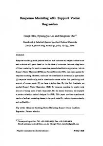
where yj is the target value for xj and f (xj ) is the prediction at xj . The computer used for these numerical experiments was PIII 866 PC with 384MB RAM and Windows 2000 as the operating system.10 7.1 Sinc Data The function sinc(x) = |x|−1 sin |x| is commonly used to illustrate SVR (Vapnik, 1995). Training and testing data sets are obtained by uniformly sampling data points from the interval [−10, 10]. Eight training data sets with sizes ranging from 50 to 4000 and a single common testing data set of 3000 cases are generated. The targets are corrupted by the noise generated by the noise model (13), using C = 10, ǫ = 0.1 and β = 0.3.11 From (15), the noise variance σn2 is 0.026785 theoretically. The true noise variances σT2 in each of the training data sets are computed and recorded in the second column of Table 3 as reference. The average squared noise in the testing data set is actually 0.026612, and the true value of average absolute noise is 0.12492. We normalize the inputs of training data sets and keep the targets unchanged. We start from the default settings with a fixed value of β = 0.3. The training results are recorded in Table 3. We find that the parameters C and ǫ approach the true value 10 and 0.1 respectively as the training sample size increases; σn2 , the variance of the additive noise that is estimated by (13) approaches σT2 too; and the ASE on testing data set also approaches the true value of average squared noise. About 60% of training samples are selected as SVs. However, the training time increases heavily as the size of training data set becomes larger. The main reason is that the number of off-bound SVs that are involved in matrix inverse becomes larger. In the next experiment, we fix β at a small value 0.1 and then carried out the training results, which are recorded in Table 4. Comparing with the case of β = 0.3, we notice that the number of off-bound SVs decreases significantly for the case β = 0.1. That reduces the computational cost for the matrix inverse in the gradient evaluation for the evidence, and hence shortens the training time greatly. Moreover, the performance in testing does not worsen. Although β is not fixed at its true value, as the the size of training data increases, the estimated variance of the additive noise σn2 still approaches σT2 and the test ASE approaches to its true value too. In order to show the function of β in our approach, we train on the 4000 data set starting from the default settings with different β ranging from 0.001 to 1.0, and plot the training results in Figure 3. We find that the number of off-bound SVs increases as β increases. The CPU time used to evaluate the evidence and its gradients increases significantly for β larger than 0.2, i.e., when the number of off-bound SVs greater than 1000. This makes the training on large-scale 10 The program bisvm.exe (version 4.2) we used for these numerical experiments can be accessed from http://guppy.mpe.nus.edu.sg/∼mpessk/papers/bisvm.zip. 11 The simulated sinc data we generated can be accessed from http://guppy.mpe.nus.edu.sg/∼chuwei/data/sinc.zip. As for how to generate the noise distributed as the model (13), refer to Appendix B.
14
data sets very slow. The introduction of β makes it possible to reduce the number of off-bound SVs that involves in matrix inverse, and then saves lots of CPU time and memory. We also find that the evidence and test ASE is slight instable in the region of very small β, meanwhile the number of off-bound SVs becomes small. One reason might be that the change on the off-bound SVs set may cause fluctuation in evidence evaluation when the number of off-bound SVs is very few. That might also result in slow convergence in the adapted SMO algorithm. Thus setting β at too small value is not desirable. There exists a large range for the value of β (from 0.01 to 0.1) where the training speed is fast and the performance is good. The introduction of β makes it possible to reduce the number of off-bound SVs that involves in matrix inverse, and hence saves lots of CPU time and memory. This is the main advantage of our approach over the classical GPR in which the inverse of the full matrix is inevitable. 7.2 Robot Arm Data The task in the robot arm problem is to learn the mapping from joint angles, x1 and x2 , to the resulting arm position in rectangular coordinates, y1 and y2 . The actual relationship between inputs and targets is as follows: y1 = 2.0 cos x1 + 1.3 cos(x1 + x2 ) and y2 = 2.0 sin x1 + 1.3 sin(x1 + x2 )
(45)
Targets are contaminated by independent Gaussian noise of standard deviation 0.05. The data set of robot arm problem we used here was generated by MacKay (1992) which contains 600 input-target pairs.12 The first 200 samples in the data set are used as training set in all cases; the second 200 samples are used as testing set; the last 200 samples are not used. Two predictors are constructed for the two outputs separately in the training. We normalize the input data and keep the original target values, and then train with Gaussian covariance function (3) and ARD Gaussian model (41) separately starting from the default settings. In the next experiment, four more input variables are added artificially (Neal, 1996), related to the inputs x1 and x2 in the original problem (45), x3 and x4 are copies of x1 and x2 corrupted by additive Gaussian noise of standard deviation 0.02, and x5 and x6 are irrelevant Gaussian noise inputs with zero mean, as follows: x1 = x1 , x2 = x2 , x3 = x1 + 0.02 · n3 , x4 = x2 + 0.02 · n4 , x5 = n5 , x6 = n6 , where n3 , n4 , n5 and n6 are independent Gaussian noise variables with zero mean and unit variance.13 We normalize the input data and keep the original target values, and then train an ARD Gaussian model (41) starting from the default settings. Their results are recorded in Table 5 ∼ Table 7.
It is very interesting to look at the training results of the ARD parameters in the case of 6 inputs in Table 7. The values of the ARD parameters show nicely that the first two inputs are most important, followed by the corrupted inputs. The ARD parameters for the noise inputs shrink very fast in training. We also record the true variance of the additive Gaussian noise on y1 and y2 in the third column of Table 6 as reference, which are about 0.0025. Although the additive noise is Gaussian that is not consistent with our loss function in likelihood evaluation, we retrieve the noise variance properly. Meanwhile we keep sparseness in solution representation. About 50% ∼ 60% of the training samples are selected as SVs (refer to Table 5).
In Table 8, we compare the test error with that in other implementations, such as neural networks with Gaussian approximation by MacKay (1992) and neural networks with Monte Carlo by Neal (1996), and Gaussian processes for regression by Williams and Rasmussen (1996). 12
The robot arm data set generated by MacKay (1992) is available at http://wol.ra.phy.cam.ac.uk/mackay/bigback/dat/. The robot arm data set with six inputs we generated can be accessed from http://guppy.mpe.nus.edu.sg/∼chuwei/data/robotarm.zip. 13
15
The expected test error of ASE based on knowledge of the true distribution is about 0.005. These results indicate that our approach gives a performance that is very similar to that given by well-respected techniques.14 7.3 Boston Housing Data The “Boston Housing” data was collected in connection with a study of how air quality affects housing prices. The data concerns the median price in 1970 of owner-occupied houses in 506 census tracts within the Boston metropolitan area. Thirteen attributes pertaining to each census tract are available for use in prediction (refer to Table 10 for details).15 The objective is to predict the median house value. Following the method used by Tipping (2000) and Saunders et al. (1998),16 the data set is partitioned into 481/25 training/testing splits randomly. This partitioning is carried out 100 times on the data.17 We normalize these training datasets to zero mean and unit variance coordinate-wise. The training with ARD model starts from the default settings and β is fixed at 0.3. The training results averaged over the 100 partitions are recorded in Table 9. The results of ARD parameters in Table 10 indicate that the most important attribute should be NOX, followed by TAX, LSTAT and RAD. We compare the test ASE result with other methods in Table 11. The performance of our approach is significantly better than that of other methods. The ARD model possesses the capacity to automatically detect the relevant attributes that improves the generalization greatly. 7.4 Laser Generated Data We use the laser data to illustrate the error bar in making predictions. The laser data has been used in the Santa Fe Time Series Prediction Analysis Competition.18 A total of 1000 points of far-infrared laser fluctuations were used as the training data and 100 following points were used as testing data set. We normalize the training data set coordinate-wise, and use 8 consecutive points as the inputs to predict the next point. We choose Gaussian kernel (3) and start training from the default settings. β is fixed at 0.3. Figure 4 plots the predictions on testing data set and the error bars. Although the predictions of our model do not match the targets very well on the region (1051-1080), the model can reasonably provide larger error bars for these predictions. This feature is very useful in other learning fields, such as active learning. 7.5 Abalone Data We use abalone data set to show the applicability and performance of our method to large data sets.19 We normalize the abalone data to zero mean and unit variance coordinate-wise, and then map the gender encoding (male/female/infant) into {(1, 0, 0), (0, 1, 0), (0, 0, 1)}. The normalized data set is split into 3000 training and 1177 testing data set randomly. The partitioning is carried out 10 times independently. The objective is to predict the abalone’s rings.20 We start from the default settings to train with Gaussian kernel (3) on the ten splits (β is fixed at 0.1). Averaging 14 Note that Monte Carlo methods sample hyperparameters hundreds of times according to P(θ|D) and then average their individual predictions. Thus they have the advantage of reducing the uncertainty in hyperparameters. On the other hand, our approach takes the mode of P(θ|D) as the optimal hyperparameters. 15 The original data can be found in StatLib, available at URL http://lib.stat.cmu.edu/datasets/boston. 16 Saunders et al. (1998) used 80 cases in 481 training data as validation set to determine the kernel parameters. 17 The 100 partitions we generated and the training results can be accessed from http://guppy.mpe.nus.edu.sg/∼chuwei/data/bostonhousing.zip. 18 Full description can be found at URL: http://www-psych.stanford.edu/ andreas/Time-Series/SantaFe.html. 19 The data can be accessed via ftp://ftp.ics.uci.edu/pub/machine-learning-databases/abalone/. 20 These partitions can be accessed from http://guppy.mpe.nus.edu.sg/∼chuwei/data/abalone.zip.
16
over the ten splits, the testing AAE is 0.4539±0.0094 and the testing ASE is 0.4354±0.0231. The CPU time consumed to evaluate the MAP estimate, evidence and its gradients once is about 89.66±5.06 seconds. 7.6 Computer Activity The computer activity database is a collection of a computer systems activity measures. The data was collected from a Sun Sparcstation 20/712 with 128 Mbytes of memory running in a multi-user university department. The final data set is a random permutation of the 8192 samples. Data for evaluating learning in valid experiments (DELVE), which is a standardized environment designed to evaluate the performance of methods that learn relationships based primarily on empirical data (Rasmussen, 1996), provides two learning tasks for the computer activity data set.21 One is to predict the portion of time that CPUs run in user mode from all attributes 1∼21, which is called “CPU” task; another is to predict the portion of time using restricted attributes (excluding the attributes 10∼18), which is named “CPUSmall” task. We choose ARD Gaussian kernel (41) and set the initial value of ARD parameters at d1 , where d is the attribute number. The initial values of other hyperparameters are chosen as the default settings, i.e. C = 1.0, ǫ = 0.05 and κb = 100.0. The data are normalized to zero mean and unit variance coordinatewise, and β is fixed at 0.3 in the training processes. The training results of the two tasks are recorded in Table 12 and Table 13, along with the results of multivariate adaptive regression splines (MARS) with bagging (Friedman, 1991; Breiman, 1994) cited from DELVE.22 If the p-value was less than 9% it is considered significant (Rasmussen, 1996). Comparing with the score of MARS provided by DELVE, the Bayesian approach to support vector regression yields overall excellant performance. In the experiments on large-scale data sets, we try our Bayesian approach on the “CPU” task, which is of 21 attributes and 8192 samples. We partitioned the computer activity data set into 7000/1192 training/testing splits randomly. This partitioning was carried out 10 times on the data set.23 We used both Gaussian covariance function (3) and ARD Gaussian (41) separately, and start from the default settings except the ARD hyperparameters at d1 , where d is the attribute number 21. β is fixed at 0.005. Their averaged results over the 10 partitions are recorded in Table 14. We find that ARD Gaussian model takes longer time, and yields quite better generalization performance. We would like to note that the last three attributes, i.e. freeswap, freemem and runqsz,24 might be the most important feature in the criterion of the ARD hyperparameters. For reasonably large-scale data sets, our Bayesian approach with the benefit of sparseness could take affordable time to achieve very good generalization.25 8. Conclusion In this chapter, we propose a Bayesian design for support vector regression using a unifying loss function. The SILF is smooth and also inherits most of the virtues of ǫ-ILF, such as insensitivity 21
The data set and its full description can be accessed at http://www.cs.toronto.edu/∼delve/data/comp-activ/. The results are obtained by the command lines: “mstats -l A -c mars3.6-bag-1” for AEL and “mstats -l S -c mars3.6bag-1” for SEL in DELVE. 23 The 10 partitions we used can be accessed from http://guppy.mpe.nus.edu.sg/∼chuwei/data/compactiv.zip. 24 According to the data description, freeswap denotes “number of disk blocks available for page swapping”, freemem denotes “number of memory pages available to user processes” and runqsz denotes “process run queue size”. 25 If we employed some scheme to cache part of the covariance matrix efficiently, the training time could be further reduced greatly. 22
17
to outliers and sparseness in solution representation. In the Bayesian framework, we integrate support vector methods with Gaussian processes to keep the advantages of both. Various computational procedures are provided for the evaluation of MAP estimate and evidence of the hyperparameters. ARD feature selection and model adaptation are also implemented intrinsically in hyperparameter determination. Another benefit is the determination of error bar in making predictions. Furthermore, sparseness in the evidence evaluation and probabilistic prediction reduces the computational cost significantly and helps us to tackle reasonably large data sets. The results in numerical experiments show that the generalization ability is competitive with other well-respected techniques. Acknowledgements Wei Chu gratefully acknowledges the financial support provided by the National University of Singapore through Research Scholarship. A. Convex Quadratic Programming Here, we give some details on how to adapt the popular SMO algorithms for classical SVR design (Smola and Sch¨olkopf, 1998; Shevade et al., 2000) to solve the convex quadratic programming problem (29), in which the constraints αi · αi∗ = 0 ∀i have been taken into consideration and pairs of variables (αi , αi∗ ) are selected simultaneously into the working set. A.1 Optimality Conditions The Lagrangian for the dual problem (29) is defined as: L=
P Pn Pn (αi − αi∗ )(αj − αj∗ )Qij − ni=1 yi (αi − αi∗ ) j=1 i=1 P P P αi∗ ) − ni=1 πi αi − ni=1 ψi αi∗ + Pni=1 (1 − β)ǫ(αi − P − ni=1 λi (C − αi ) − ni=1 ηi (C − αi∗ ) 1 2
(46)
where Qij = Cov(xi , xj ) + δij 2βǫ with δij the Kronecker delta. Let us define C Fi = yi −
n X j=1
(αj − αj∗ )Q(xi , xj )
(47)
and the KKT conditions should be: ∂L ∂αi
= −Fi + (1 − β)ǫ − πi + λi = 0 πi ≥ 0, πi αi = 0, λi ≥ 0, λi (C − αi ) = 0, ∀i ∂L = Fi + (1 − β)ǫ − ψi + ηi = 0 ∂α∗i ψi ≥ 0, ψi αi∗ = 0, ηi ≥ 0, ηi (C − αi∗ ) = 0, ∀i These conditions can be simplified by considering five cases for each i: Case 1 : αi = αi∗ = 0 −(1 − β)ǫ ≤ Fi ≤ (1 − β)ǫ Case 2 : αi = C Fi ≥ (1 − β)ǫ Case 3 : αi∗ = C Fi ≤ −(1 − β)ǫ Case 4 : 0 < αi < C Fi = (1 − β)ǫ ∗ Case 5 : 0 < αi < C Fi = −(1 − β)ǫ 18
(48)
We can classify any one pair into one of the following five sets, which are defined as: I0a = {i : 0 < αi < C} I0b = {i : 0 < αi∗ < C} I0 = I0a ∪ I0b I1 = {i : αi = αi∗ = 0} I2 = {i : αi∗ = C} I3 = {i : αi = C}
(49)
Let us denote Iup = I0 ∪ I1 ∪ I3 and Ilow = I0 ∪ I1 ∪ I2 . We further define Fiup on the set Iup as ½ Fi + (1 − β)ǫ if i ∈ I0b ∪ I1 up Fi = Fi − (1 − β)ǫ if i ∈ I0a ∪ I3 and Filow on the set Ilow as Filow
=
½
Fi + (1 − β)ǫ if i ∈ I0b ∪ I2 Fi − (1 − β)ǫ if i ∈ I0a ∪ I1
Then the conditions in (48) can be simplified as Fiup ≥ 0 ∀i ∈ Iup and Filow ≤ 0 ∀i ∈ Ilow Thus the stopping condition can be compactly written as: bup ≥ −τ and blow ≤ τ
(50)
where bup = min{Fiup : i ∈ Iup }, blow = max{Filow : i ∈ Ilow }, and the tolerance parameter τ > 0, usually 10−3 . If (50) holds, we reach a τ -optimal solution. At the optimal solution, the training samples whose index i ∈ I0 are off-bound SVs, on-bound SVs if i ∈ I2 ∪ I3 , and non-SVs if i ∈ I1 . A.2 Sub-optimization Following the design proposed by Keerthi et al. (2001), we employ the two-loop approach till the stopping condition is satisfied. We update two Lagrange multipliers towards the optimal values in either Type I or Type II loop every time. In the Type II loop we update the pair associated with bup and blow , while in the Type I loop either bup or blow is chosen to be updated together with the variable which violates KKT conditions. The algorithm has been summarized in Table 1 in which the stopping condition is defined as in (50). Now we study the solution to the sub-optimization problem, i.e. how to update the violating pair. Suppose that the pair of the Lagrangian multipliers being updated are {αi , αi∗ } and {αj , αj∗ }. The other Lagrangian multipliers are fixed during the updating. Thus, we only need to find the minimization solution to the sub-optimization problem. In comparison with the sub-optimization problem in classical SVR, the only difference lies in that the sub-optimization problem cannot be analytically solved here. We could choose Newton-Raphson formulation to update the two Lagrangian multipliers. Since only two variables in the sub-optimization problem, there is no need for matrix inverse. The sub-optimization problem can be stated as n
min
αi ,α∗i ,αj ,α∗j
n
1 XX (αi′ − αi∗′ )(αj ′ − αj∗′ )Qi′ j ′ − (αi − αi∗ )yi − (αj − αj∗ )yi + (1 − β)ǫ(αi + αi∗ + αj + αj∗ ) 2 i′ =1 j ′ =1 19
SMO Initialization
Type I Loop Type II Loop
Switcher
Termination
Table 1. The main loop in SMO algorithm. Algorithm BOOL CheckAll = TRUE ; BOOL Violation = TRUE ; choose any α and α ∗ that satisfy 0 ≤ αi ≤ C and 0 ≤ α∗i ≤ C vote the current bup and blow While ( CheckAll == TRUE or Violation == TRUE ) if ( CheckAll == TRUE ) check optimality condition one by one over all samples update the violating pair and then set Violation = TRUE else while (the stopping condition does not hold) update the pair associated with bup and blow ; vote bup and blow within the set I0 endwhile set Violation = FALSE endif if (CheckAll == TRUE) set CheckAll = FALSE elseif (Violation == FALSE) set CheckAll = TRUE endif endwhile return α, α ∗
subject to 0 ≤ αi ≤ C, 0 ≤ αi∗ ≤ C, 0 ≤ αj ≤ C and 0 ≤ αj∗ ≤ C, where Qi′ j ′ = Cov(xi′ , xj ′ ) + with δi′ j ′ the Kronecker delta.26 We need to distinguish four different cases: (αi , αj ), δi′ j ′ 2βǫ C ∗ (αi , αj ), (αi∗ , αj ), (αi∗ , αj∗ ), as that in Figure 5. It is easy to derive the unconstrained solution to the sub-optimization problem according to Newton-Raphson formulation. The unconstrained solutions are tabulated in Table 2 with ρ = Qii Qjj − Qij Qij , Gi = −Fi + (1 − β)ǫ, Gj = −Fj + (1 − β)ǫ, G∗i = Fi + (1 − β)ǫ, G∗j = Fj + (1 − β)ǫ, where Fi is defined as in (47). Table 2. Unconstrained solution in the four quadrants. Quadrant I (αi , αj ) II (αi∗ , αj ) III (αi∗ , αj∗ ) IV (αi , αj∗ )
Unconstrained Solution αinew αinew αinew αinew
= αi + (−Qjj Gi + Qij Gj )/ρ = αi + (−Qjj G∗i − Qij Gj )/ρ = αi + (−Qjj G∗i + Qij G∗j )/ρ = αi + (−Qjj Gi − Qij G∗j )/ρ
αjnew αjnew αjnew αjnew
= αj = αj = αj = αj
+ (Qij Gi − Qii Gj )/ρ + (−Qij G∗i − Qii Gj )/ρ + (Qij G∗i − Qii G∗j )/ρ + (−Qij Gi − Qii G∗j )/ρ
It may be happened that for a fixed pair of indices (i, j) the initial chosen quadrant, say e.g. (αi , αj∗ ) is the one with optimal solution. In a particular case the other quadrants, (αi , αj ) and even (αi∗ , αj ), have to be checked. It occurs (see Figure 5) if one of the two variables hits the 0 boundary, and then the computation of the corresponding values for the variables with(out) asterisk according to the following table is required. Moreover, there is no need to solve the suboptimization problem exactly that requires lot of iterations. In practice, we use Newton-Raphson formulation once only to check the applicable quadrants.27 In numerical experiments, we find that the adapted algorithm can efficiently find the solution at nearly the same computational cost as that required by SMO in classical SVR.28 ½
1 if i = j . 0 otherwise 27 There is no significant reduction in computational cost when we use Newton-Raphson formulation in iterative way to find the exact solution of the sub-optimization problem. 28 The source code can be accessed at http://guppy.mpe.nus.edu.sg/∼chuwei/code/bisvm.zip. The routines in bismo routine.cpp and bismo takestep.cpp were written in ANSI C to solve the quadratic programming problem. 26
The Kronecker delta is defined as δij =
20
B. Noise Generator Given a random variable u with a uniform distribution in the interval (0, 1), we wish to find a function g(u) such that the distribution of the random variable z = g(u) is a specified function Fz (z). We maintain that g(u) is the inverse of the function u = Fz (z): if z = Fz−1 (u), then P(z ≤ z) = Fz (z) (refer to Papoulis (1991) for a proof).
Given the probability density function PS (δ) as in (13), the corresponding distribution function should be 1 ∗ exp(C(δ + ǫ)) CZS ¸ if δ ∈ ∆C · q ³q ´ πβǫ C 1 1 if δ ∈ ∆M ∗ erf (δ + (1 − β)ǫ) C 4βǫ 2 − ZS (1 − β)ǫ − 1 + ZδS if δ ∈ ∆0 (51) F (δ) = 2 · q ³q ´¸ 1 C if δ ∈ ∆M + Z1S (1 − β)ǫ + πβǫ erf (δ − (1 − β)ǫ) 2 C 4βǫ if δ ∈ ∆C 1.0 − CZ1 S exp(−C(δ − ǫ)) Now we solve the inverse problem to sample data in the distribution (51): given a uniform distribution of u in the interval (0, 1), we let δ = Fδ−1 (u) so that the distribution of the random variable δ equals to the distribution (51). References Bishop, C. M. Neural Networks for Pattern Recognition. Oxford University Press, 1995. Breiman, L. Bagging predictors. Technical Report 421, Department of Statistics, University of California, Berkeley, California, USA, 1994. Buntine, W. L. and A. S. Weigend. Bayesian back-propagation. Complex Systems, 5(6):603–643, 1991. Byrd, R. H., P. Lu, and J. Nocedal. A limited memory algorithm for bound constrained optimization. SIAM Journal on Scientific and Statistical Computing, 16(5):1190–1208, 1995. Chu, W., S. S. Keerthi, and C. J. Ong. A unified loss function in Bayesian framework for support vector regression. In Proceeding of the 18th International Conference on Machine Learning, pages 51–58, 2001. http://guppy.mpe.nus.edu.sg/∼mpessk/svm/icml.pdf. Duane, S., A. D. Kennedy, and B. J. Pendleton. Hybrid Monte Carlo. Physics Letters B, 195 (2):216–222, 1987. Evgeniou, T., M. Pontil, and T. Poggio. A unified framework for regularization networks and support vector machines. A.I. Memo 1654, Massachusette Institute of Technology, 1999. Fletcher, R. Practical methods of optimization. John Wiley and Sons, 1987. Friedman, J. H. Multivariate adaptive regression splines (with discussion). Annals of Statistics, 19(1), 1991. Gao, J. B., S. R. Gunn, C. J. Harris, and M. Brown. A probabilistic framework for SVM regression and error bar estimation. Machine Learning, 46:71–89, March 2002. Huber, P. J. Robust Statistics. John Wiley and Sons, New York, 1981. Keerthi, S. S. and S. K. Shevade. SMO algorithm for least squares SVM formulations. Technical Report CD-02-08, Dept. of Mechanical Engineering, National University of Singapore, http://guppy.mpe.nus.edu.sg/∼mpessk/papers/lssvm smo.ps.gz, 2002. 21
Keerthi, S. S., S. K. Shevade, C. Bhattacharyya, and K. R. K. Murthy. Improvements to Platt’s SMO algorithm for SVM classifier design. Neural Computation, 13:637–649, March 2001. Kimeldorf, G. S. and G. Wahba. Some results on Tchebycheffian spline function. Journal of Mathematical Analysis and Applications, 33:82–95, 1971. Kwok, J. T. The evidence framework applied to support vector machines. IEEE Transactions on Neural Networks, 11(5):1162–1173, 2000. Lampinen, J. and A. Vehtari. Bayesian approach for neural networks - reviews and case studies. Neural Networks, 14:257–274, 2001. Law, M. H. and J. T. Kwok. Bayesian support vector regression. Proceedings of the Eighth International Workshop on Artificial Intelligence and Statistics (AISTATS), pages 239–244, 2001. Key West, Florida, USA. Luenberger, D. G. Linear and Nonlinear Programming. Addison-Wesley Publishing Company, Menlo Park, California, 2nd edition, 1984. MacKay, D. J. C. A practical Bayesian framework for back propagation networks. Neural Computation, 4(3):448–472, 1992. MacKay, D. J. C. Bayesian methods for backpropagation networks. Models of Neural Networks III, pages 211–254, 1994. MacKay, D. J. C. Probable networks and plausible predictions - a review of practical Bayesian methods for supervised neural networks. Network: Computation in Neural Systems, 6(3): 469–505, 1995. Micchelli, C. A. Interpolation of scatter data: Distance matrices and conditionally positive definite functions. Constructive Approximation, 2:11–22, 1986. Neal, R. M. Bayesian training of backpropagation networks by the hybrid Monte Carlo method. Technical Report CRG-TR-92-1, Department of Statistics, University of Toronto, 1992. Neal, R. M. Bayesian Learning for Neural Networks. Lecture Notes in Statistics. Springer, 1996. Papoulis, A. Probability, Random Variables, and Stochastical Processes. McGraw-Hill, Inc., New York, 3rd edition, 1991. Pontil, M., S. Mukherjee, and F. Girosi. On the noise model of support vector regression. A.I. Memo 1651, Massachusetts Institute of Technology, Artificail Intelligence Laboratory, 1998. Rasmussen, C. E. Evaluation of Gaussian processes and other methods for non-linear regression. Ph.D. thesis, University of Toronto, 1996. Saunders, C., A. Gammerman, and V. Vovk. Ridge regression learning algorithm in dual variables. In Proceedings of the 15th International Conference on Machine Learning, pages 515– 521, 1998. Sch¨olkopf, B., R. Herbrich, and A. J. Smola. A generalized representer theorem. In Proceedings of the Annual Conference on Computational Learning Theory, 2001. Seeger, M. Bayesian model selection for support vector machines, Gaussian processes and other kernel classifiers. In Advances in Neural Information Processing Systems, volume 12, 1999. Shevade, S. K., S. S. Keerthi, C. Bhattacharyya, and K. R. K. Murthy. Improvements to the SMO algorithm for SVM regression. IEEE Transactions on Neural Networks, 11:1188–1194, Sept. 2000. Smola, A. J. and B. Sch¨olkopf. A tutorial on support vector regression. Technical Report NC2-TR-1998-030, GMD First, October 1998. 22
Sollich, P. Bayesian methods for support vector machines: Evidence and predictive class probabilities. Machine learning, 46:21–52, 2002. Tipping, M. E. The relevance vector machine. Advances in Neural Information Processing Systems 12, pages 652–658, 2000. MIP Press. Vanderbei, R. J. Linear Programming: Foundations and Extensions, volume 37 of International Series in Operations Research and Management Science. Kluwer Academic, Boston, 2nd edition, June 2001. Vapnik, V. N. The Nature of Statistical Learning Theory. New York: Springer-Verlag, 1995. Wahba, G. Spline Models for Observational Data, volume 59 of CBMS-NSF Regional Conference Series in Applied Mathematics. SIAM, 1990. Williams, C. K. I. Prediction with Gaussian processes: from linear regression to linear prediction and beyond. Learning and Inference in Graphical Models, 1998. Kluwer Academic Press. Williams, C. K. I. and C. E. Rasmussen. Gaussian processes for regression. In Touretzky, D. S., M. C. Mozer, and M. E. Hasselmo, editors, Advances in Neural Information Processing Systems, volume 8, pages 598–604, 1996. MIT Press.
23
Quadratic Loss Function
Laplacian Loss Function
2
2
1.5
1.5
1
1
0.5
0.5
0
0
−2
−1
0
1
2
−2
Huber’s Loss Function
0
1
2
Epsilon Insensitive Loss Function
2
2
1.5
1.5
1
1
0.5
0.5
0 −3
−1
0 −2
−1
0
ε
2
3
−3
−2
−1
0
ε
2
3
Figure 1. Graphs of popular loss functions, where ǫ is set at 1.
1 0.9 0.8
Soft Insensitive Loss Function
0.7 0.6 0.5 0.4 0.3 0.2
Noise Distribution
0.1 0 −1.5
∆M*
∆C* −1
−(1+β)ε
−0.5
∆ο −(1−β)ε
0
∆M (1−β)ε ε=0.5
∆C (1+β)ε
1
1.5
Figure 2. Graphs of soft insensitive loss function (solid curve) and its corresponding noise density function (dotted curve), where ǫ = 0.5, β = 0.5 and C = 2.0 in the noise model.
24
Number of Support Vectors
Average CPU Time in Seconds for an Evaluation 350
4000
300 3000
250
SVs
200
2000 150
for MAP estimate 100
1000
off−bound SVs 0 −3 10
−2
10
50
−1
10
β
for gradient evaluation
0 −3 10
0
10
−2
10 −6
Negative Logarithm of the Evidence −1620
15
−1625
−1
β
0
10
10
Test ASE Minus True Value
x 10
10
−1630 5 −1635 0
−1640 −1645 −3 10
−2
10
−1
β
−5 −3 10
0
10
the true value of ASE 0.026612
10
−2
10
−1
β
0
10
10
Figure 3. Graphs of training results with respect to different β for the 4000 sinc data set. The horizontal axis indicates the value of β in log-scale. The solid line in upper left graph indicates the number of SVs, while the dotted line indicates the number of off-bound SVs. In the upper right graph, the solid line indicate the CPU time in seconds used to evaluate evidence and its gradient, and the dotted line is the CPU time in seconds consumed for MAP estimate. In the lower left graph, the dots indicate − ln P(D|θ) in training results. In the lower right graph, the dots indicate the average squared error (ASE) in testing minus the true value in the additive noise that is 0.026612.
Table 3. Training results on sinc data sets with the fixed value of β = 0.3. σT2 denotes the true value of noise variance in training data set; σn2 denotes the noise variance in training data retrieved by (13); − ln P(D|θ) denotes the negative log evidence of the hyperparameters as in (37); SVM denotes the number of off-bound support vectors; SVC denotes the number of on-bound support vectors; TIME denotes the CPU time in seconds consumed in the training; AAE is the average absolute error in testing; ASE denotes the average squared error in testing; the true value of average squared noise in the testing data set is 0.026612; the true value of average absolute noise in the testing data set is 0.12492. Size
σT2
C
ǫ
σn2
κ
− ln PD|θ
SVM
SVC
Time
AAE
ASE
50 100 300 500 1000 2000 3000 4000
.03012 .03553 .02269 .02669 .02578 .02639 .02777 .02663
15.95 10.00 11.16 9.36 9.90 10.01 9.96 10.51
.181 .136 .118 .080 .094 .096 .106 .111
.02416 .03152 .02478 .02752 .02655 .02630 .02770 .02609
5.19 5.85 5.57 5.89 5.62 5.01 5.20 5.76
-1.3 -11.1 -113.7 -174.8 -389.9 -808.8 -1146.7 -1642.2
23 33 90 135 270 539 833 1226
4 25 87 218 388 768 1052 1280
0.15 0.40 5.95 12.9 63.0 436.2 1551.4 3291.9
.13754 .13027 .12642 .12544 .12537 .12509 .12511 .12501
.031194 .028481 .027189 .026765 .026834 .026661 .026671 .026615
25
300 250 200 150 100 50 0 −50 1000
1010
1020
1030
1040
1050 1060 time series
1070
1080
1090
1100
1010
1020
1030
1040
1050 1060 time series
1070
1080
1090
1100
30 20 10 0 −10 −20 1000
Figure 4. Graphs of our predictions on laser generated data. In the upper graph, the dots indicate our predictions on the testing data set and the solid curve describes the time series. In the lower graph, p the dot indicates estimation error that is equal to prediction minus target, and solid curves indicate the error bars ±2 σt2 + σn2 in predictive distribution.
Table 4. Training results on sinc data sets with the fixed value of β = 0.1. σT2 denotes the true value of noise variance in training data set; σn2 denotes the noise variance in training data retrieved by (13); b denotes the bias term in regression function defined as in (10); − ln P(D|θ) denotes the negative log evidence of the hyperparameters as in (37); SVM denotes the number of off-bound support vectors; SVC denotes the number of on-bound support vectors; TIME denotes the CPU time in seconds consumed in the training; AAE is the average absolute error in testing; ASE denotes the average squared error in testing; the true value of average squared noise in the testing data set is 0.026612; the true value of average absolute noise in the testing data set is 0.12492. Size
σT2
C
ǫ
σn2
κ
− ln PD|θ
SVM
SVC
Time
AAE
ASE
50 100 300 500 1000 2000 3000 4000
.03012 .03553 .02269 .02669 .02578 .02639 .02777 .02663
6.70 12.07 12.05 9.42 9.96 10.06 9.96 10.41
.086 .163 .124 .080 .095 .096 .108 .109
.05018 .02855 .02300 .02715 .02631 .02600 .02774 .02623
9.42 5.54 5.92 5.78 6.09 5.06 5.34 5.74
5.51 -10.1 -113.8 -174.4 -389.7 -808.5 -1142.6 -1643.3
10 19 39 57 102 190 287 446
20 25 100 250 459 920 1303 1650
0.11 0.53 5.13 9.43 47.9 264.7 1070.4 2852.3
.13411 .13366 .12651 .12543 .12540 .12512 .12509 .12502
.030065 .029728 .027212 .026764 .026848 .026662 .026673 .026619
26
Table 5. Training results on robot arm data set with the fixed value of β = 0.3. SVM denotes the number of off-bound support vectors; SVC denotes the number of on-bound support vectors; TIME denotes the CPU time in seconds consumed in the training; EVAL denotes the times of the evaluations on evidence and its gradients required by the optimization package; UNIT denotes the CPU time in seconds consumed for an evaluation on evidence and its gradients; NMSE denotes the normalized mean squared error. AAE(10
−2
)
ASE(10
−3
)
NMSE(10
−3
Kernel
y
SVM
SVC
Time
Eval
Unit
Gaussian with 2 inputs
y1 y2
70 75
37 28
53.8 83.7
31 27
1.7 3.1
4.032 4.765
2.586 3.375
2.045 1.046
ARD Gaussian with 2 inputs
y1 y2
74 75
27 47
27.3 61.1
19 17
1.4 3.6
3.892 4.552
2.457 3.162
1.943 0.980
Gaussian with 6 inputs
y1 y2
125 128
11 5
32.3 68.2
21 20
1.5 3.4
7.422 6.070
13.774 6.421
10.893 1.990
ARD Gaussian with 6 inputs
y1 y2
69 76
33 47
39.0 82.4
24 21
1.6 3.9
3.880 4.609
2.450 3.207
1.937 0.994
)
Table 6. Training results on the two-dimensional robot arm data set with the fixed value of β = 0.3. σT2 denotes the true value of noise variance in the training data; σn2 denotes the estimated value of the noise variance. σT2
Kernel
y
Gaussian with 2 inputs
y1 y2
ARD Gaussian with 2 inputs
y1 y2
(10−3 )
C
ǫ
2.743 2.362
35.61 44.07
0.048 0.050
2.743 2.362
39.05 36.79
0.052 0.039
σn2
(10−3 )
κ
κb
2.913 2.368
0.467 0.486
23.39 12.77
2.809 2.399
κ1 =0.665; κ2 =0.237 κ1 =0.657; κ2 =0.188
10.39 14.56
Table 7. Training results on the six-dimensional robot arm data set with the fixed value of β = 0.3. σn2 denotes the estimated value of the noise variance; UNIT denotes the CPU time in seconds consumed for an evaluation on evidence and its gradients; NMSE denotes the normalized mean squared error. y
C
ǫ
y1 y2
36.70 36.39
.049 .037
σn2
(10−3 )
2.878 2.373
κ1
κ2
.712 .771
.222 .161
κ3 (10
−2
.199 6.09
)
κ4 (10
−2
)
.185 1.15
κ5 (10
−5
)
0.01 0.01
κ6 (10
−5
0.01 0.01
)
κb 8.09 10.73
Table 8. Comparison with other implementation methods on testing ASE of the robot arm positions. INPUTS denotes the number of inputs. ASE denotes the average squared error in testing. IMPLEMENTATION METHOD
INPUTS
ASE
2 2
5.73 5.57
Hybrid Monte Carlo of Neal
2 6
5.47 5.49
Gaussian Processes of Williams
2 6
5.63 5.69
Our method with ARD Gaussian Covariance Function
2 6
5.62 5.66
Gaussian Approximation of MacKay Solution with highest evidence Solution with lowest test error
27
Table 9. Training results on Boston housing data set with the fixed value of β = 0.3. Time denotes the CPU time in seconds consumed for training on one partition; NMSE denotes the normalized mean squared error. The results are computed by averaging over the 100 partitions and its standard deviations are also computed. − ln P(D|θ)
C
ǫ
Time
AAE
ASE
164.6±9.5
9.83±0.40
0.144±0.015
52.2±11.9
1.85±0.36
6.90±4.40
NMSE(10
−2
)
8.80±5.23
Table 10. Training results of ARD hyperparameters on Boston housing data set with the fixed value of β = 0.3. The results are computed by averaging over the 100 partitions and its standard deviations are also computed. Attribute
Description
ARD
CRIM ZN INDUS CHAS NOX RM AGE DIS RAD TAX PTRATIO B LSTAT
per capita crime rate by town proportion of residential land zoned for lots over 25,000 sq. ft proportion of non-retail business acres per town Charles River dummy variable (1 if tract bounds river; 0 otherwise) nitric oxides concentration (parts per 10 million) average number of rooms per dwelling proportion of owner-occupied units built prior to 1940 weighted distances to five Boston employment centers index of accessibility to radial highways full-value property-tax rate per $10,000 pupil-teacher ratio by town 1000(Bk−0.63)2 where Bk is the proportion of blacks by town % lower status of the population
0.0363±0.0126 0.0142±0.0043 0.0659±0.0150 0.0329±0.0185 3.6681±1.6795 0.1415±0.0274 0.0417±0.0105 0.1231±0.0275 0.2400±0.0409 0.9418±0.3511 0.0428±0.0083 0.0306±0.0135 0.2421±0.1120
Table 11. Comparison with Ridge Regression (Saunders et al., 1998) and Relevance Vector Machine Tipping (2000) on price prediction of the Boston Housing data set. ASE denotes the average squared test error. IMPLEMENTATION METHOD
KERNEL TYPE
ASE
Ridge Regression Ridge Regression Ridge Regression Relevance Vector Machine Our Method
Polynomial Splines ANOVA Splines Gaussian ARD Gaussian
10.44 8.51 7.69 7.46 6.90
Table 12. Training results on CPU task of the computer activity data set from DELVE. MARS denotes multivariate adaptive regression splines with bagging; BSVR denotes the Bayesian approach to support vector regression we proposed; AEL denotes the standardized estimated expected loss using absolute error loss; SEL denotes the standardized estimated expected loss using squared error loss; p-value denotes the p-value of the t-test computed by DELVE. We use the bold face to indicate the cases in which p-value satisfied the threshold 0.09. Size
MARS AEL
BSVR AEL
p-value
MARS SEL
BSVR SEL
p-value
64 128 256 512 1024
1.4203±0.5393 1.0571±0.3769 0.2826±0.0069 0.2680±0.0092 0.2593±0.0142
0.4306±0.0521 0.2910±0.0173 0.2488±0.0205 0.1996±0.0047 0.1758±0.0030
0.1000 0.0793 0.1608 0.0010 0.0096
45.7003±37.4136 64.0895±57.0036 0.0432±0.0037 0.0434±0.0111 0.0351±0.0078
0.3113±0.1058 0.1144±0.0230 0.0682±0.0178 0.0283±0.0031 0.0182±0.0016
0.2644 0.2987 0.1614 0.2917 0.0870
28
Table 13. Training results on CPU task of the computer activity data set from DELVE. MARS denotes multivariate adaptive regression splines with bagging; BSVR denotes the Bayesian approach to support vector regression we proposed; AEL denotes the standardized estimated expected loss using absolute error loss; SEL denotes the standardized estimated expected loss using squared error loss; p-value denotes the p-value of the t-test computed by DELVE. We use the bold face to indicate the cases in which p-value satisfied the threshold 0.09. Size
MARS AEL
BSVR AEL
p-value
MARS SEL
BSVR SEL
p-value
64 128 256 512 1024
5.4524±2.6336 2.0377±1.2582 0.8819±0.3372 0.2763±0.0054 0.2690±0.0078
0.4851±0.0547 0.3348±0.0171 0.2832±0.0176 0.2414±0.0045 0.2216±0.0039
0.1017 0.2169 0.1249 0.0004 0.0145
3059.2593±2361.2878 808.4435±798.4149 87.5683±73.1864 0.0357±0.0013 0.0339±0.0019
0.3444±0.1182 0.1226±0.0202 0.0710±0.0169 0.0384±0.0039 0.0300±0.0024
0.2363 0.3450 0.2708 0.4827 0.3287
Table 14. Training results on CPU task of the computer activity data set with 7000 training samples. β is fixed at 0.005. SVM denotes the number of off-bound SVs; SVC denotes the number of on-bound SVs; TIME denotes the CPU time in hours consumed by the training on a partition; σn2 denotes the estimated noise variance in the normalized targets; AAE denotes averaged absolute test error; ASE denotes averaged squared test error.
Gaussian ARD
SVM
SVC
Time
σn2
AAE
ASE
1082.3±107.9 847.0±156.3
2823.1±381.8 2910.4±725.6
3.14±1.06 5.88±1.61
0.0216±0.0052 0.0100±0.0016
2.008±0.102 1.633±0.055
11.320±3.015 5.830±1.027
Figure 5. Possible quadrant changes of the pair of the Lagrange multipliers.
29