Response Modeling with Support Vector Regression
Dongil Kim, Hyoung-joo Lee and Sungzoon Cho ∗ Department of Industrial Engineering, Seoul National University, San 56-1, Shillim-dong, Kwanak-gu, Seoul, 151-744, Korea
Abstract Response modeling, which predicts whether each customer will respond or how much each customer will spend based on the database of customers, becomes a key factor of direct marketing. In previous researches, several classification approaches, include Support Vector Machines (SVM) and Neural Networks (NN), have been applied for response modeling. However, there are two drawbacks of conventional approaches: (1) response models only predict classification scores rather than predicting total amount of money spent, (2) too large training data. For the first drawback, we applied Support Vector Regression (SVR) for response modeling to predict total amount of money spent of each respondent. For the second drawback, we employed a pattern selection method designed for SVR. This paper provides experimental results of a direct marketing dataset in terms of model fit, training time complexity and profitability. Key words: Response Modeling, Direct Marketing, Support vector machines; Regression; Pattern selection
∗ Corresponding author. Tel: +82-2-883-4913, Fax: +82-2-883-4913 Email addresses:
[email protected] (Dongil Kim),
[email protected]
Preprint submitted to Elsevier Science
26 May 2006
1
Introduction
A response model, given a mailing campaign, predicts whether each customer will respond or how much each customer will spend based on the database of customers’ demographic information and/or purchase history. Marketers will send mails or catalogs to customers who are predicted to respond or to spend large amounts of money. A well-targeted mail increases the profit, while a mistargeted or unwanted mail not only increases the marketing cost but also may worsen the customer’s relationship to the firm (G¨on¨ ul et al., 2000; Potharst et al., 2000). Various methods have been used for response modeling such as statistical techniques (Bentz and Merunka, 2000; Haughton and Oulabi, 1997; Ling and Li, 1998; Suh et al., 1999), machine learning techniques, (Wang et al., 2005; Chiu, 2002; Cheung et al., 2003; Shin and Cho, 2006; Viaene el al., 2001; Yu and Cho, 2005) and neural networks (NN) (Potharst et al., 2000; Bentz and Merunka, 2000; Zahavi and Levin, 1997). So far, a response model have been usually formulated as a binary classification problem because of its straightforwardness. The customers are divided into two classes, respondents and non-respondents. A classifier is constructed to predict whether a given customer will respond or not. From a modeling point of view, however, as pointed out in (KDD98 Cup, 1998) for the KDD-CUP-98 task, there is an inverse correlation between the likelihood to buy and the dollar amount to spend (Wang et al., 2005). This is because the more dollar amount is involved, the more cautious the customer is in making a purchase decision. In this sense, the likelihood to buy that is estimated by a classification model may not lead to more profit. Therefore, in addition to the classification approach, a regression model needs to be applied for response modeling to (Hyoung-joo Lee),
[email protected] (Sungzoon Cho).
2
predict total amount of money of each customer. Support Vector Machine (SVM) is known as the most spot-lighted algorithm with great generalization performances by employing Structural Risk Minimization (SRM) principle (Vapnik, 1995). Support Vector Regression (SVR), a regression version of SVM was developed to estimate regression functions (Druker et al., 1997). Like SVM, SVR is capable of solving non-linear problems using kernel functions and successful in various domains (Druker et al., 1997; M¨ uller et al., 1997). However, there was a difficulty to train SVR on real-world dataset. As the number of training patterns increases, SVR training takes much longer with a time complexity of O(N 3 ) where N denotes the number of training patterns. So far, many algorithms such as Chunking, SMO, SVMlight and SOR have been proposed to reduce the training time. However, their training time complexity is still strongly related to the number of training patterns (Platt, 1999). We take another direction called pattern selection which is focusing on reducing the number of training patterns. NPPS (Shin and Cho, 2003) is a proved method of pattern selection for SVM, but it’s only for SVM classifiers. Rather we use a pattern selection method based on ε-tube which is especially designed for SVR (Kim and Cho, 2006). In this paper, we applied SVR for response modeling to predict total amount of money spent of each respondent. As mentioned before, a single response model based on classification method can score the likely to respond of each customer. However, direct marketers would like to know not only respondents but also profitable customers who will spend more money than others. Hence, after predicting respondents by a classification response model, a regression model is needed to predict total amount of money spent of each respondent. As the classification model was not our concerned, we supposed there was a primitive ideal classifier which could find all respondents without False Posi3
Fig. 1. The ideal procedure of the paper. Especially, the paper is focused on the two dark boxes.
tive (FP) errors. We made a subset consists of only but all respondents from original dataset. SVR model was applied to the subset of respondents. The ideal procedure of this paper is presented in Fig 1. We used the DMEF4 dataset from the Direct Marketing Educational Foundation (DMEF) which is collected from a catalog mailing task. The remaining of this paper is organized as follows. In Section 2, we introduce the concepts of SVR and provide the main idea of the pattern selection method with a simple toy example. In Section 3, we present details of DMEF datasets and parameters for experiment. In Section 4, experiment results are following. In section 5, we summarize the result and conclude the paper with a remark on limitations and future research directions.
2
Pattern Selection for Support Vector Regression
2.1 Support Vector Regression
For a brief review of SVR, consider a regression function f(x) to be estimated with training patterns {(xi , yi )}, f (x) = w · x + b with w, x ∈ RN , b ∈ R 4
(1)
where {(x1 , y1 ), · · · , (xn , yn )} ∈ RN × R
(2)
SVR is moved around to include training patterns inside ε-insensitive tube (ε-tube). By the SRM principle, the generalization accuracy is optimized by the flatness of the regression function. Since the flatness is guaranteed on a small w, SVR is moved to minimize the norm, kwk2 . An optimization problem could be formulated with constraints where C, ε, and ξ, ξ ∗ are trade-off cost between empirical error and the flatness, size of ε-tube and slack variables, respectively, for the following soft margin problem. n X 1 kwk2 + C (ξi + ξi∗ ), 2 i=1 Subject to yi − w · xi − b ≤ ε + ξi , w · xi + b − yi ≤ ε + ξi∗ , ξi , ξi∗ ≥ 0, i = 1, · · · , n.
Minimize
(3)
Hence, SVR is trained by minimizing kwk2 with including training patterns inside the ε-tube. With adding Lagrangian multipliers α and α∗ , the QP problem can be optimized as dual problem. The estimated regression function from SVR is following where ns is the number of support vectors:
f (x) =
ns X
(α − α∗ )K(xi , x) + b
(4)
i=1
2.2 Pattern Selection for Support Vector Regression
The training time complexity of SVR is O(N 3 ). If the number of training patterns increases, the training time increases more radically, i.e. in a cubic proportion. Marketing databases usually consists of over one millions of customers and hundreds of input variables. Hence, it takes too long time to train SVR directly to marketing dataset. We applied a pattern selection method from our previous research (Kim and Cho, 2006). 5
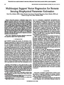
Fig. 2. (a) The regression function after training original dataset, and (b) the regression function after training ONLY patterns inside estimated ε–tube.
SVR trains patterns based on ε-loss function foundation. SVR makes ε-tube on the training patterns. The patterns in ε-tube are not counted as error, and patterns out of ε-tube, i.e. Support Vectors (SVs), are used for training. In addition, SVR estimates the regression function as the center-line of ε-tube. Hence, if ε-tube can be estimated before training, we can find the regression function with only those patterns inside ε-tube (See Fig. 2) . However, removing all patterns outside ε-tube could lead to reduction of ε-tube itself, thus it is desirable to keep some of “outside” patterns for training. Hence, we defined a “fitness” probability for each pattern based on its location with respect to ε-tube and then selected patterns stochastically. We made k bootstrap samples of size l (l < n) from original training pattern set (D). We trained an SVR with each bootstrap sample and obtained k SVR regression functions. Each regression function was used to see if a training pattern is located inside ε-tube. Each training pattern in D is located inside a minimum of zero ε-tubes to a maximum of k ε-tubes. Let mj denote the number of times that pattern j is found in-side an ε-tube. We use mj as the likelihood that pattern j is actually located inside the real ε-tube. Each mj is converted to a probability, pj as in Eq. (5). Since we want to select patterns 6
Fig. 3. (a) Original dataset and an SVR trained on it, (b) A bootstrap sample and an SVR trained on it, (c) Original dataset and ε-tube of (b)’s SVR, and (d) Selected patterns and an SVR trained on them
inside ε-tube, pattern j is selected with a probability of pj ,
mj . pj = Pn i=1 mj
(5)
The procedure of the pattern selection method is presented in Fig. 3 with a simple toy example. The algorithm is presented in Fig. 4. 7
1.
Initialize the number of bootstrap samples, k Initialize the number of patterns in each bootstrap sample, l Initialize the number of patterns to be selected, s
2.
Make k bootstrap samples, Di , (i = 1, · · · , k), from the original dataset D by random sampling without replacement
3. 4.
Train SVR fi with Di , (i = 1, · · · , k) Count the number of times mj that pattern j is found inside ε-tube of fi
5. 6.
Convert mj to pj according to Eq. (5) Select s patterns stochastically from D without replacement based on pj
7.
Train final SVR with s selected patterns Fig. 4. ε-tube based pattern selection algorithm
3
Dataset and Experimental Settings
3.1 Dataset: DMEF dataset
We utilized DMEF4 dataset which contains 101,532 customers and 91 input variables. The response rate is 9.4% with 9,571 respondents and 91,961 nonrespondents. We selected a subset based on the weighted dollars used from previous researches (Yu and Cho, 2005; Ha et al., 2005). We would like to design a regression model as a scoring model after picking up respondents with a primary classification model. Since a classification model was not our 8
Table 1 Input variables Name
Formulation
Description
ORIGINAL VARIABLES Purseas
Number of seasons with a purchase
Falord
LTD fall orders
Ordtyr
Number of orders this year
Puryear
Number of years with a purchase
Sprord
LTD spring orders Derived Variables
DERIVED VARIABLES Recency
Order days since 10/1992
Tran53
I(180 ≤ recency ≤ 270)
Tran54
I(270 ≤ recency ≤ 366)
Tran55
I(366 ≤ recency ≤ 730)
Tran38
1/recency
Comb2
P14
m=1 ProdGrpm
Number of product groups purchased from this year
Tran46
√ comb2
Tran42
log(1 + ordtyr × falord)
Interaction between the number of orders
Tran44
√ ordhist × sprord
Interaction between LTD orders and LTD spring orders
Tran25
1/(1+lorditm)
Inverse of latest-season items
interest in this research, we assumed that there was an ideal response model built with a classification algorithm that could pick all respondent without false acceptances. Hence, we selected a new dataset consists of customers only whose target dollars are positive, i.e. only respondents. The final selected dataset consists of 4,000 customers. For performance evaluation, the dataset was partitioned into training and 9
test sets. A half of customers were randomly assigned to the training set while the other half to the test set. Performance of a model shows a large variation with regard to a specific data split (Malthouse, 2002). So ten different training/test splits were generated. All results are averaged of each exclusive training/tes sets. We are not interested in feature selection/extraction. Malthouse extracted 17 input variables for this dataset and Ha et al (Ha et al., 2005) used 15 out of them, removing two variables whose variations are negligible. In this paper, these 15 variables were used as input variables as listed in Table 1. We formulated this dataset to a regression problem by setting the total amount of dollars as target variable.
3.2 Experimental Settings
We made three different response models based on SVR in the experiments. All experimental results of SVR with pattern selection (SVR-PS) were compared with results of SVR with all data (SVR-100) and SVR with random sampling (SVR-Random). We set hyper-parameters of SVR. The hyper-parameters of SVR were determined by cross–validation for SVR-100 with C × ε = {0.1, 1, 5, 10, 50, 100} × {0.01, 0.05, 0.07, 0.1, 0.5, 0.7, 1}. RBF kernel was used as a kernel function and the kernel parameter σ was fixed to 1.0 for all datasets. The parameters of the pattern selection method were set as follows. In this case, the number of bootstrap samples k was set to 10. The other parameter that controls the number of patterns in a bootstrap sample l was set to 25% of the number of patterns in dataset, n. The number of selected patterns was set to 10% to 90% of n. During the experiments, we used all data as normalized vectors. Root Mean Squared Error (RMSE) is used to estimate the model fits. We calculated the 10
averaged profits per one catalog mail to estimate the profitability of response models. Also we recorded training times. All stochastic results were the averaged values of 10-time repeats.
4
Experimental Results
4.1 Model Fit and Time Complexity
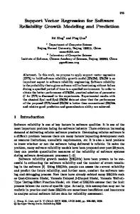
Fig. 5 shows the experimental results. The solid lines present the result of SVR with all data (SVR-100). The lines with circles presents the results of SVR with pattern selection (SVR-PS) while the lines with boxes presents the results of SVR with random sampling (SVR-Random). Fig. 5 (a) is RMSEs which have real values (dollars). It shows SVR-PS is slightly less accurate than SVR-100, but is significantly more accurate than SVR-Random. As more patterns were selected, the training dataset became similar to the original dataset and the gaps between all SVRs became narrower. With 10% pattern selection, the gap of RMSEs between SVR-PS and SVR-Random is larger than 15 dollars. When the percentage of selected patterns is 40% of all, the gaps of RMSEs between SVR-PS and SVR-100 are less than 5 dollars. Fig. 5 (b) shows averaged training time of all SVRs. It takes 1200 seconds to train all data with SVR. However, with 10% of pattern selection, SVR-PS needed only 16% of training time of SVR-100. Although the percentage of selected patterns was up to 40%, which resulted only 5 dollars’ gap, SVR-PS needed only 25% of training time of SVR-100. SVR-PS is more efficient than SVR-100. 11
85
SVR−100 SVR−PS SVR−Random
RMSE
80
75
70
65
60
55 10
20
30
40
50
60
70
80
90
80
90
Percentage of patterns selected (%) (a) 1400 1200
Time (sec)
1000
SVR−100 SVR−PS SVR−Random
800 600 400 200 0 10
20
30
40
50
60
70
Percentage of patterns selected (%) (b) Fig. 5. (a) RMSE resulted from experiments and (b) the training times
12
150
150
SVR−100 SVR−PS SVR−Random
130 120 110 100 90 80 70 60 50
SVR−100 SVR−PS SVR−Random
140
Average profit per mail ($)
Average profit per mail ($)
140
130 120 110 100 90 80 70 60
0.1
0.2
0.3
0.4
0.5
0.6
0.7
Mailing depth (%)
0.8
0.9
50
1
0.1
0.2
0.3
0.4
(a)
0.7
0.8
0.9
1
150
SVR−100 SVR−PS SVR−Random
130
SVR−100 SVR−PS SVR−Random
140
Average profit per mail ($)
140
Average profit per mail ($)
0.6
(b)
150
120 110 100 90 80 70 60 50
0.5
Mailing depth (%)
130 120 110 100 90 80 70 60
0.1
0.2
0.3
0.4
0.5
0.6
0.7
Mailing depth (%)
0.8
0.9
1
50
0.1
0.2
(c)
0.3
0.4
0.5
0.6
0.7
Mailing depth (%)
0.8
0.9
(d)
Fig. 6. Average profit per one mail. (a) Results of 10% pattern selection and random sampling, from (b) to (d) are 30%, 50%, 70% respectively
4.2 Profitability
Fig. 6 compares three response models of SVR in terms of profit. For each setting, the response model predicted the dollar amount to each test customer. Then, we sorted the test customers by descending order in terms of the dollar amount predicted by model. A mailing depth of Fig. 6 is an expected profit made in a promotion to each percentage of top-decile. As it shows, if we send catalog mails to all respondents, the averaged profit of each mail is roughly 13
1
60 dollars. However, if we want to select 10% of all respondents, we can make more profit based on SVR model than only use classification model. As mailing depths go larger, averaged profits per mail decrease. SVR-PS resulted between SVR-100 and SVR-Random. As we saw the training time complexity analysis in Fig. 5 (b), SVR-PS guaranteed efficient models with acceptable profitability and fast training speed.
5
Conclusions and Discussion
We applied SVR for response modeling. We assumed that there was a previous response model that could find all respondents, perfectly. With SVR, we estimated total amount of dollar spent for each customer to find more profitable respondents. As results, we could find high profit customers rather than just response rate. Also, to reduce the training time complexity, we used the pattern selection method. The pattern selection method made SVR be an efficient model and, at the same time, avoid worsening the accuracy. SVR-100 resulted the best and SVR-Random resulted the worst in terms of accuracy and profit, while SVR-Random resulted the best in terms of training speed. SVR-PS located a reasonable area in terms of efficiency which guarantees accurate like SVR-100 and fast like SVR-Random. SVR-PS needs only 16∼25% of training time of SVR-100, with acceptable accuracy loss. There are some limitations of this research. First, it was an early research of applying SVR for response modeling. We formulated the problem as a regression form, however, we might have missed some key factors of data setting for regression formulation. With further researches, we can find more effective regression formulation to be applied response modeling. Second, the results of SVR-PS looked efficient, however, we couldn’t decide those were good 14
enough to apply real-world problems. The pattern selection method should be improved to be more accurate. Finally, various experiments including profit analysis should be followed in further study. We assumed there was a perfect classification model, however, there will be a comparison with the real classification model in further study.
References Bentz, Y., Merunka D., 2000. Neural networks and the multinomial logit for brand choice modeling: a hybrid approach, Journal of Forecasting 19, 177200. Cheung, K.-W., Kwok, J.T., Law, M.H., Tsui, K.-C., 2003.mining customer product ratings for personalized marketing, Decision Support Systems 35, 231-243. Chiu, C., 2002.a case-based customer classification approach for direct marketing, Expert Systems with Applications 22(2), 163-168. Drucker, H., Burges, C. J. C., Kaufman, L., Smola, A., Vapnik, V., 1997.Support Vector Regression Machines, In: Mozer, M. C., Jordan, M. I., Petsche, T.(eds.): Advances in Neural In-formation Processing System 9, MIT Press, Cambridge, MA, 155-161. G¨on¨ ul, F.F., Kim, B.D., Shi, M., 2000. Mailing smarter to catalog customer, Journal of Interactive Marketing 14(2), 2-16. Ha, K., Cho, S., MacLachlan, D., 2005.Response models based on bagging neural networks, Journal of Interactive Marketing 19(1), 17-30. Haughton, D., Oulabi, S., 1997.Direct marketing modeling with CART and CHAID, Journal of Direct Marketing 11(4), 42-52. KDD98, The KDD-CUP-98 result, 1998. http://www.kdnuggets.com/ meetings/kdd98/kdd-cup-98.html. 15
Kim, D., Cho, S., 2006.ε-tube based Pattern Selection for Support Vector Machines Lecture Notes in Artificial Intelligence 3918, 215-224. Ling, C.X., Li, C., 1998.Data mining for direct marketing: problems and solutions, Proceedings of ACM SIGKDD International Conference on Knowledge Discovery and Data Mining (KDD-98), New York, pp. 73-79. Malthouse, E.C., 2002.Performance-based variable selection for scoring models. Journal of Interactive Marketing 16(4), 37-50. M¨ uller K.-R., Smola A., R¨atsch G., Sch¨olkopf B., Kohlmorgen J., Vapnik V., 1997.Predicting time series with support vector machines. In: GerstnerW., Germond A., Hasler M., and Nicoud J.-D. (Eds.), Artificial Neural Networks ICANN97, Berlin. Lecture Notes in Computer Science 1327, 999-1004. Platt, J. C., 1999.Fast Training of Support Vector Machines Using Sequential Minimal Optimization, Advanced in Kernel Methods; Support Vector Machines, MIT Press, Cambridge, MA, pp. 185-208. Potharst, R., Kaymak, U., Pijls W., 2000. Neural networks for target selection in direct marketing, Erasmus Research Institute of Management (ERIM), RSM Erasmus University, Research Paper ERS-2001-14-LIS, Available at http://ideas.repec.org/s/dgr/eureri.html. Shin, H., Cho, S., 2003.Fast Pattern Selection Algorithm for Support Vector Classifiers: Time Complexity Analysis, Lecture Notes in Computer Science 2690, 1008-1015. Shin, H., Cho, S., 2006.Response modeling with support vector machines, Expert Systems with Applications 30(4), 746-760. Suh, E.H., Noh, K.C., Suh, C.K., 1999.Customer listsegmentation using the combined response model, Expert Systems with Applications 17(2), 89-97. Vapnik, V., 1995. The Natural of Statistical Learning Theory, Springer, New York. Viaene, S., Baesens, B., Gestel, T., Suykens, J.A.K., 2001.Van den Poel, D.,
16
Vanthienen, J., De Moor, B., Dedene, G., Knowledge discovery in a direct marketing case using least squares support vector machines, International Journal of Intelligent Systems 16, 1023-1036. Wang, K., Zhou, S., Yang, Q., Yeung, J.M.S., 2005. Mining customer value: from association rules to direct marketing, Data Mining and Knowledge Discovery 11, 57-79. Yu, E., Cho, S., 2005.Constructing response model using ensemble based on feature subset selection, Expert Systems with Applications, In Press, Available online at http://www.sciencedirect.com/science/journal/ 09574174. Zahavi, J., Levin, N, 1997.Applying neural computing to target marketing. Journal of Direct Marketing 11(4), 76-93.
17