Received: 27 September 2017
Revised: 28 April 2018
Accepted: 29 April 2018
DOI: 10.1002/bimj.201700182
R E S E A R C H PA P E R
Bayesian variable selection logistic regression with paired proteomic measurements Alexia Kakourou
Bart Mertens
Department of Medical Statistics and Bioinformatics, Leiden University Medical Center, 2300 RC Leiden, The Netherlands Correspondence Alexia Kakourou, Department of Medical Statistics and Bioinformatics, Leiden University Medical Center, 2300 RC Leiden, The Netherlands. Email:
[email protected] Funding information MEDIASRES, Grant/Award Number: 290025
Abstract We explore the problem of variable selection in a case-control setting with mass spectrometry proteomic data consisting of paired measurements. Each pair corresponds to a distinct isotope cluster and each component within pair represents a summary of isotopic expression based on either the intensity or the shape of the cluster. Our objective is to identify a collection of isotope clusters associated with the disease outcome and at the same time assess the predictive added-value of shape beyond intensity while maintaining predictive performance. We propose a Bayesian model that exploits the paired structure of our data and utilizes prior information on the relative predictive power of each source by introducing multiple layers of selection. This allows us to make simultaneous inference on which are the most informative pairs and for which— and to what extent—shape has a complementary value in separating the two groups. We evaluate the Bayesian model on pancreatic cancer data. Results from the fitted model show that most predictive potential is achieved with a subset of just six (out of 1289) pairs while the contribution of the intensity components is much higher than the shape components. To demonstrate how the method behaves under a controlled setting we consider a simulation study. Results from this study indicate that the proposed approach can successfully select the truly predictive pairs and accurately estimate the effects of both components although, in some cases, the model tends to overestimate the inclusion probability of the second component. KEYWORDS added-value assessment, Bayesian variable selection, isotope clusters, mass spectrometry, paired measurements, prediction
1
I N T RO D U C T I O N
Proteomics is the large-scale study of proteins that aim to provide a better understanding of the function of cellular and disease processes at the protein level. The most widely used technology to assess proteomic expression is mass spectrometry that has undergone remarkable evolution over the last 20 years. Particularly ultrahigh-resolution mass spectrometers (MS) such as Fourier-transform MS have become the most powerful and efficient tools for the quantitative analysis of complex protein mixtures in biological systems.
This is an open access article under the terms of the Creative Commons Attribution License, which permits use, distribution and reproduction in any medium, provided the original work is properly cited. © 2018 The Authors. Biometrical Journal published by WILEY-VCH Verlag GmbH & Co. KGaA, Weinheim. Biometrical Journal. 2018;1–18.
www.biometrical-journal.com
1
KAKOUROU AND MERTENS
2
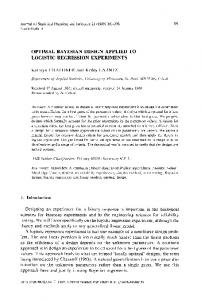
FIGURE 1
(A) A mass spectrum for a single individual. (B) An isotopic cluster at position m/z 2021,2
Irrespective of its type, a mass-spectrometer takes as input a molecular mixture and outputs a so-called mass spectrum. A mass spectrum (as shown in Figure 1A) is a sequence of intensity readings distributed over a mass-to-charge (m/z) range, generated from the detection of ionized molecules. In ultrahigh-resolution mass spectrometry, each species (such as peptide) is detected and expressed as a “density” of isotope peaks (as shown in Figure 1B)—rather than a single peak—in the mass spectrum, resulting from the distribution of naturally occurring elements. The peaks of an isotopic density represent ions of the same elemental composition but different isotopic composition due to the presence of additional neutrons in their nucleus. We commonly refer to these isotopic densities as isotopic clusters. The late improvements in mass spectrometry technologies, and thus the quality of the acquired data, turned the focus of recent research toward methods for optimally processing and interpreting high-resolution mass spectral data (at the individual level) using knowledge on the properties of the isotope densities (such as peak detection algorithms or deisotoping methods). However, the predictive potential of the isotopic cluster information, inherent in such data, has not been fully exploited yet. At date, a common practice for summarizing the proteomic expression (for example so that it can be later used for prediction purposes) is to use information on the amount of expression (intensity). In a recent work, Kakourou, Vach, Nicolardi, van der Burgt, and Mertens (2016) proposed an alternative approach to using the relative intensity level for summarizing the predictive information within isotope clusters in individual mass spectra. Recognizing
KAKOUROU AND MERTENS
3
that an isotope cluster is a density, they proposed to use, apart from information on the intensity, information on the shape of the isotopic clusters in order to translate the isotopic expression into cluster summaries that could be later used as new predictors for the construction of diagnostic rules. Shape-based summary measures aim to estimate the shape of either directly the observed isotopic cluster pattern or, alternatively, the deviation of that observed pattern from the typical pattern (as defined in Kakourou et al., 2016). Using the proposed summary measures (based on either intensity or shape information) as new input variables (separately) into a prediction model, the authors showed that both types of information are predictive of the health status of an individual, though intensity has greater predictive capacity as compared to shape. Having established the presence of an overall isotope cluster effect as well as a shape effect in addition to intensity effect, our aim in this work is twofold: (a) to identify a collection of isotope clusters associated with the disease outcome and (b) to optimally integrate the two sources of information. We wish to address these questions in a way that allows us to assess the added-value of shape beyond intensity in predicting the class outcome of an individual while maintaining predictive performance. Several approaches have been proposed in the literature to address the problem of variable selection in the prediction of binary outcomes, with Lasso regularization (Tibshirani, 1996) being among the most popular ones. The lasso uses a l1 -norm constraint on the vector of regression coefficients that shrinks the parameter estimates toward zero while it induces sparsity in the model. An extension of the lasso, introduced as “group lasso” was proposed (Meier, van de Geer, and Bhlmann, 2008) to perform variable selection on (predefined) groups of variables in logistic regression models. This procedure is a regularization algorithm that acts like the lasso at the group level. Depending on the amount of regularization, an entire group of predictors may drop out of the model. If the groups are all of size one, the group lasso reduces to the lasso. A key limitation of the group lasso is that it does not yield sparsity within a group. That is, if a group of variables is included in the model then all variables within that group are attributed a nonzero effect. For problems with grouped covariates, Simon, Friedman, Hastie, and Tibshirani (2012) considered a more general penalty, termed “sparse-group lasso,” which yields sparsity at both the group and individual variables levels, in order to select groups as well as predictors within a group. The proposed penalty is a convex combination of the lasso and group lasso penalties that results in both “group-wise sparsity” and “within-group sparsity.” While the sparse-group lasso has been reported to give favorable results in prediction and classification problems, it selects within-group predictors without taking into account any prior knowledge on the relative importance of each individual predictor in the group. Given that such prior (or expert) knowledge exists, a more suitable/interesting approach would be to introduce some type of hierarchy in the selection process, for example by prioritizing selection of specific predictors that have already proven their predictive value in previous applications. This would additionally allow us to assess the complementary predictive potential of “secondary” predictors after accounting for “primary” predictors (the term is used with respect to their established predictive capacity, cost of measuring etc.). The problem of assessing the added-value of a secondary predictor on top of a primary predictor in the high-dimensional setting has been considered by Boulesteix and Hothorn (2010) and by Rodríguez-Girondo et al. (in press). Boulesteix and Hothorn proposed a permutation-based testing procedure for assessing the additional predictive value of high-dimensional molecular data on top of clinical predictors through combinations of logistic regression and boosting methods. Rodríguez-Girondo et al. introduced a two-stage approach for the assessment of the added predictive ability of omic predictors, based on sequential crossvalidation and regularized regression models. However, both of these approaches are used to evaluate whether there is additional predictive information in a secondary source after correcting for a primary source at a “global level,” hence they do not address the question of where does the extra predictive information come from (which specific predictors within the secondary source, if any, carry additional information on the outcome) or how large is the additional contribution of any individual predictor from the secondary source. In this paper, we propose an approach that can explore the problem of isotope selection and at the same time address the problem of assessing the additional predictive value of the shape source over and above the intensity source. Our approach uses a Bayesian model formulation that exploits the paired structure of the proteomic data and utilizes prior knowledge on the relative predictive power of each individual source to assess the added-value of shape, by introducing multiple layers of selection. In doing so, the Bayesian model makes the explicit assumption that the shape source is complementary. In terms of model fitting, this is translated by assuming that a shape measure can be included in the set of predictors on the condition that it is accompanied by/coupled with its corresponding intensity while the reverse does not need to hold. This assumption allows us to make simultaneous inference on which isotope clusters are the most informative with respect to the class outcome and for which isotopes—and most importantly to what extent—shape has a complementary value in separating the two groups. The remainder of this paper is organized as follows: We first introduce the pancreatic cancer data and their paired structure that is a key component of these particular data. The problem of isotope selection, on the one hand, and assessment of the added-value of shape, on the other, through a Bayesian model formulation is explored next. We then present results from applying the Bayesian model to the pancreatic cancer data consisting of the paired intensity-shape measurements. Results from the analysis
KAKOUROU AND MERTENS
4
of the fitted model show that most predictive potential is achieved with a subset of just 6 (out of 1289) pairs, which are consistently selected with very high probability of inclusion, while the contribution of the intensity components is much higher than the shape components. We explore the relative performance and the degree of agreement (with respect to the selected isotope clusters) between our method and an alternative approach based on a stability selection strategy utilizing sparse-group lasso. Additionally, we show a simulation example to demonstrate how the proposed method behaves under a controlled setting. The outcome of the simulation study indicates that the proposed approach can successfully select the truly predictive pairs and accurately estimate the effects of both components although, in some cases, the model tends to overestimate the inclusion probability of the second component. We finish with a discussion.
2
DATA
In this paper, we reanalyze data from a case-control study that was carried out at the Leiden University Medical Centre (Nicolardi et al., 2014). The study involved 273 individuals, consisting of 88 pancreatic cancer patients and 185 healthy volunteers. The samples collected from those individuals were distributed over three MALDI-target plates and thereafter mass analyzed by a MALDI-FTICR MS system, giving rise to a single mass spectrum for each sample within the mass range of 1013–3700 Da (full details on the design and measurement protocol can be found in Nicolardi et al., 2014). In previous work (Kakourou et al., 2016), the authors applied to the pancreatic cancer data a peak detection algorithm in order to identify the isotopic clusters and their corresponding peaks. As a result, the complete proteomic expression in the individual spectra was reduced to clusters of isotopic expression on which summary measures could be defined. To derive the cluster summaries the authors proposed to use information on either the intensity or the shape of the observed isotope cluster pattern. In this work, rather than considering single measurements of intensity or shape as our predictor variables, we recognize intensity and shape are tied together and regard them as paired measurements such that the components of each predictor pair represent cluster summaries of isotopic expression based on intensity information, in the case of the first component, and shape information, in the case of the second. The intensity component of a pair is denoted in the following by 𝑢 and is defined as the sum of log-transformed peak intensities 𝑙𝑗 , 𝑗 = 1, … , 𝐽 within an isotope cluster (where 𝐽 denotes the number of peaks in a cluster and is cluster-specific), given by ∑ 𝑙𝑗 (1) 𝑢 ∶= 𝑗
The shape component, denoted by 𝑣, is defined as 𝑣 ∶=
∑ 𝑗
𝑗𝑝𝑗
the center of gravity of a distribution on the values 1, … , 𝐽 , where 𝑝𝑗 ∶=
(2) 𝑥𝑗 ∑ 𝑗 𝑥𝑗
and 𝑥1 , … , 𝑥𝐽 denote the residuals that measure
the deviation of the observed isotopic pattern from the typical pattern. For a more detailed description on how these summary measures were created/derived we refer the interested readers to Kakourou et al. (2016). We choose these particular summary measures to represent the intensity-based and shape-based components due to their superiority, as compared to other proposed summary measures, with regard to their individual predictive ability. Our final dataset consists of 1289 pairs of intensity and shape summary measures. Our objective is to investigate whether we can develop methods to integrate both types of information in a way that will allow us to calibrate more interpretable rules and/or learn more about the interplay between intensity and shape in predicting the class outcome, while maintaining predictive performance.
3 3.1
BAYES IAN VA R I A B L E - SE L E C TIO N M O DEL O N PA IRS The logistic regression model
Let the data be given by (𝒚, 𝒛), where 𝒚 = (𝑦1 , … , 𝑦𝑛 )⊺ is the binary case-control outcome with 𝑦𝑖 ∈ {0, 1} for 𝑖 = 1, … , 𝑛 independent individuals while 𝒛 = (𝒛1 , … , 𝒛𝑛 )⊺ represents the predictor source with each 𝒛𝑖 = ((𝑢𝑖1 , 𝑣𝑖1 ), … , (𝑢𝑖𝑝 , 𝑣𝑖𝑝 )) consisting of a sequence of paired intensity and shape measurements for 𝑝 isotope clusters. We consider the binary regression model 𝑦𝑖 ∼ Benoulli(𝑝𝑖 )
(3)
KAKOUROU AND MERTENS
5
with logit(𝑝𝑖 ) = 𝛽0 + 𝒛𝑖 𝜷
(4)
where 𝑝𝑖 is the case-probability for the 𝑖-th observation and 𝜷 = ((𝑎1 , 𝑏1 ), … , (𝑎𝑝 , 𝑏𝑝 )) represents the vector of paired regression parameters with the first and second elements of each pair corresponding to the effects of the intensity and shape measurements respectively.
3.2
Variable-dimension logistic regression model
We assume that only a subset of isotope clusters is relevant for predicting the class outcome and that 𝒖 is expected to carry more information on the class outcome than 𝒗. Our main objective is to assess the added-value of the shape source 𝒗 on top of the intensity source 𝒖 in predicting the health status of future patients. Under the assumption that only a set of isotope clusters is predictive of the health status of an individual, the true model is given by logit(𝑝𝑖 ) = 𝛽0 + 𝒛̃ 𝑖 𝜷̃ = ( ) ( ) ( ) = 𝛽0 + 𝑎̃1 𝑢̃ 𝑖1 + 𝑏̃ 1 𝑣̃𝑖1 + 𝑎̃2 𝑢̃ 𝑖2 + 𝑏̃ 2 𝑣̃𝑖2 + ⋯ + 𝑎̃𝑘 𝑢̃ 𝑖𝑘 + 𝑏̃ 𝑘 𝑣̃𝑖𝑘 = = 𝛽0 +
(5)
𝑘 ∑ ( ) 𝑎̃𝑗 𝑢̃ 𝑖𝑗 + 𝑏̃ 𝑗 𝑣̃𝑖𝑗 𝑗=1
where 𝒛̃ = ((𝑢̃ 1 , 𝑣̃1 ), … , (𝑢̃ 𝑘 , 𝑣̃𝑘 )) represents the unknown set of paired measurements that are associated with the class outcome with regression coefficient vector 𝜷̃ = ((𝑎̃1 , 𝑏̃ 1 ), … , (𝑎̃𝑘 , 𝑏̃ 𝑘 )) that is of unknown dimension 𝑘 ≤ 𝑝. The isotope dimensionality 𝑘 is thus considered/treated as a parameter in the model and will be estimated from the data along with the unknown set of intensity-shape pairs and their corresponding regression coefficients. In order to assess the added-value of shape information over and above intensity information we place a logical constraint on the inclusion of shape information that specifies that if 𝑎 = 0 then 𝑏 = 0 (if 𝑏 ≠ 0 then 𝑎 ≠ 0). The above formulation suggests that shape can be included in the model only on the condition that its corresponding intensity is included as well. Note that the reverse is not true. Hence, rather than forcing mutual selection of both components of the isotope pairs we let the data decide whether the first component (intensity) alone provides all the required information for separating the two groups. With this constraint, (5) reduces to
logit(𝑝𝑖 ) = 𝛽0 +
𝑘𝐶 𝑘𝐼 ∑ ( ) ∑ 𝑎̃𝑗 𝑢̃ 𝑖𝑗 + 𝑏̃ 𝑗 𝑣̃𝑖𝑗 + 𝑎̃𝑙 𝑢̃ 𝑖𝑙 𝑗=1
(6)
𝑙=1
where 𝑘𝐶 denotes the dimensionality of the “complete” isotope couples and indicates how many times a shape measure is included in the model in conjunction with its corresponding intensity and 𝑘𝐼 denotes the dimensionality of intensity singletons so that 𝑘 = 𝑘𝐼 + 𝑘𝐶 .
3.3
Prior specification
To complete the model formulation, we have to specify the prior structure for all the model parameters. For the intercept we assume a weakly informative normal prior 𝛽0 ∼ 𝑁(0, 102 ). We specify independent normal priors on the regression parameters 𝑎̃𝑗 ∼ 𝑁(0, 𝜎𝑎2 ) and 𝑏̃ 𝑗 ∼ 𝑁(0, 𝜎𝑏2 ), for 𝑗 = 1, … , 𝑘 and 𝑏𝑗 ≠ 0, where the variances 𝜎𝑎2 = 𝜏𝑎2 𝑐𝑎 and 𝜎𝑏2 = 𝜏𝑏2 𝑐𝑏 control the magnitude of included effects for intensity and shape respectively, 𝜏𝑎 and 𝜏𝑏 are known rescaling factors while 𝑐𝑎 = 1∕𝑠𝑎 and 𝑐𝑏 = 1∕𝑠𝑏 are randomly distributed scale factors with gamma priors placed on 𝑠𝑎 and 𝑠𝑏 . Under the above prior assumption on the regression parameters, the covariance matrix Σ has a block-diagonal structure with block matrices along the diagonal of the [ 𝜎2 0 ] form Σ𝑗 = 𝑎 2 , if 𝑏𝑗 ≠ 0, and Σ𝑗 = 𝜎𝑎2 otherwise. The prior specification is completed by assigning a prior to the isotope 0
𝜎𝑏
dimension parameter 𝑘. We use a discrete uniform prior on the set of integers {0, 1, 2, … , 𝑘𝑚𝑎𝑥 } with 𝑘𝑚𝑎𝑥 a large positive integer corresponding to the maximum allowed isotope dimension.
KAKOUROU AND MERTENS
6
3.4
MCMC model fitting
We present an adaptation of the reversible jump MCMC implementation described in Mertens (2016) for fitting the logistic model, in order to perform isotope selection, on the one hand, and assess the added-value of shape beyond intensity, on the other. Evaluation of the added-value of shape is achieved by introducing a second layer of shape selection on top of the isotope selection. Our MCMC sampler is based on a random choice between three basic move steps: (1) BIRTH, (2) DEATH, and (3) CHANGE. The first two of these steps propose moves between different isotope dimensions while the last one proposes moves within an isotope dimension and between different variable dimensions. More specifically, in the BIRTH step, we propose with probability 𝑏𝑘 = 1∕3 to add a new randomly chosen isotope into the model set. In the DEATH step, we propose with probability 𝑑𝑘 = 1∕3 to remove a randomly chosen isotope from the current model set. Shape selection is facilitated by splitting each of these steps into two additional substeps such that, in the case of a BIRTH move proposal, we may choose between proposing to add either the entire pair (couple) into the model, with probability = 𝑏𝑘 ∕2, or solely the first component of the pair (intensity), with probability 𝑏𝐼𝑘 = 𝑏𝑘 ∕2. Note that the candidate set from 𝑏𝐶 𝑘 which we may select a new isotope is the set containing all “complete” isotopes that do not currently have any component in the model set. Analogously, in the case of a DEATH move proposal, we may choose between proposing to remove either a complete isotope (couple) from the current set, with probability 𝑑𝑘𝐶 = 𝑑𝑘 ∕2, or an intensity singleton, with probability 𝑑𝑘𝐼 = 𝑑𝑘 ∕2. Apart from the BIRTH and DEATH steps that propose moves between isotope dimensions by either adding or removing isotopes (singletons or pairs) to and from the current set, we may propose to change the composition of an isotope already included in the model, with probability 𝑐𝑘 = 1∕3. We do so by introducing a CHANGE step. Again here, within this step, we may choose between two substeps that either change an isotope couple into an intensity singleton that is remove shape from the included isotope pair, with probability 𝑐𝑘𝐶→𝐼 = 𝑐𝑘 ∕2, or change an intensity singleton into an isotope couple that is add shape to the included intensity singleton, with probability 𝑐𝑘𝐼→𝐶 = 𝑐𝑘 ∕2. In this way, we give a second chance to shape selection/deselection by allowing the data to judge whether a shape measure contributes to classification in addition to intensity and thus should join its corresponding intensity or does not provide any additional information over and above intensity and therefore could be omitted from the isotope pair in the model set. We choose 𝐼 = 𝑑(𝑘=𝑘 𝑏𝐼(𝑘=0) = 𝑏𝐶 (𝑘=0)
𝑚𝑎𝑥 =𝑘𝐼 )
𝐼 𝑑(0