Input variable selection for median flood ... - Wiley Online Library

WATER RESOURCES RESEARCH, VOL. 47, W07503, doi:10.1029/2011WR010436, 2011

Input variable selection for median flood regionalization W. Z. Wan Jaafar,1 J. Liu,1 and D. Han1 Received 18 January 2011; revised 31 March 2011; accepted 14 April 2011; published 2 July 2011.

[1] Flood estimation for ungauged catchments is a challenging task for hydrologists. A modern geographical information system is able to extract a large number of catchment characteristics as input variables for regionalization analysis. Effective and efficient selection of the best input variables is urgently needed in this field. This paper explores a new methodology for selecting the best input variable combination on the basis of the gamma test and leave‐one‐out cross validation (LOOCV) to estimate the median annual maximum flow (as an index flood). Since the gamma test is capable of efficiently calculating the output variance on the basis of the input without the need to select a model structure type, more effective regionalization models could be developed because there is no need to define an a priori model structure. A case study from 20 catchments in southwest England has been used to illustrate and validate the proposed scheme. It has been found that the gamma test is able to narrow down the search options to be further explored by the LOOCV. The best formula from this approach outperforms the conventional approaches based on cross validation, data filtering with Spearman’s rank correlation matrix, and corrected Akaike information criterion. In addition, the developed formula is significantly more accurate than the existing equation used in the Flood Estimation Handbook. Citation: Wan Jaafar, W. Z., J. Liu, and D. Han (2011), Input variable selection for median flood regionalization, Water Resour. Res., 47, W07503, doi:10.1029/2011WR010436.

1. Introduction [2] Accurate estimation of floods is an important component in designing hydraulic structures such as dams, spillways, culverts, water supply systems, and other flow control structures. Flood estimation at ungauged catchments has always been a challenging problem for hydrologists. The regionalization technique is usually applied to estimate flow statistics using catchment morphometric and climatic characteristics. An assumption of this technique is that flood characteristics can be explained by catchment characteristics [Mazvimavi et al., 2005]. With the regionalization approach, many researchers have developed regression models for estimating floods using catchment characteristics [Natural Environment Research Council, 1975; Canuti and Moisello, 1982; Acreman, 1985; Mimikou and Gordios, 1989; Garde and Kothyari, 1990; Reimers, 1990]. The use of regression models to forge a link between a certain hydrological parameter to a set of catchment characteristics is a long‐established practice in hydrology because of the simple nature of the regression models and the relatively limited data requirement compared with more detailed hydrological models [Kjeldsen and Jones, 2009]. Many case studies relating hydrological parameters to catchment characteristics in a statistical manner have been carried out by the hydrological community [Rodríguez‐Iturbe, 1969; Jakeman et al., 1992; Sefton et al., 1 Water and Environmental Management Research Centre, Department of Civil Engineering, University of Bristol, Bristol, UK.

Copyright 2011 by the American Geophysical Union. 0043‐1397/11/2011WR010436

1995; Post and Jakeman, 1996; Abdulla and Lettenmaier, 1997; Post et al., 1998; Sefton and Howarth, 1998; Seibert, 1999; Fernandez et al., 2000; Lamb et al., 2000; Lamb and Kay, 2004; Merz and Blöschl, 2004; Wagener et al., 2004; Wagener and Wheater, 2006]. However, despite of decades of research in this field, there are still several potential difficulties in flood regionalization: (1) it is not always easy to get the required data for model development, (2) there are no effective and efficient selection methods for input variables (or sometime called independent variable which are not always correct in the real world since they may correlate with each other to a certain degree), (3) even if input variables are chosen, it is hard to find a suitable model structure, and (4) model parameter estimation is not always easy because of the inadequacy of the available data. [3] In the United Kingdom, the [Centre for Ecology and Hydrology (CEH), 1999] has provided a large number of catchment characteristics (Flood Estimation Handbook, FEH) which are derived from hydrologically adjusted soil maps, land use maps, CEH digital terrain maps, etc.. Those maps are specific for the United Kingdom and not easily obtainable by flood researchers elsewhere. It is important that alternative catchment characteristics based on more widely available digital maps and data sets should be explored. Nowadays, more data and digital maps are open to academic research and geographic information system (GIS) is a powerful tool for researchers to extract the required information. In this study, we attempt to create a different set of catchment characteristics and make comparisons with the FEH catchment descriptors (“catchment descriptor” is a name used in the FEH to describe catchment characteristics).

W07503

1 of 18

W07503

WAN JAAFAR ET AL.: VARIABLE SELECTION FLOOD REGIONALIZATION

[4] With the extracted catchment characteristics, the follow‐up problem is how to choose a set of input variables for the regionalization model development. With GIS and modern digital maps, large number of catchment characteristics can be extracted and it is not always straightforward to decide the most effective input variables. Variable selection refers to the problem of selecting input variables that are most predictive of a given outcome [Guyon and Elisseeff, 2003]. In computer science, the important reasons for variable selection have been discussed by Leray and Gallinari [1999], including that they can reduce the amount of data to be collected or processed, make model training easier, improve model estimates using relevant features on small data sets, and improve model performance by avoiding the interference of nonrelevant information. The benefits of effective variable selection can be summarized as: facilitating data visualization and data understanding, reducing the measurement and storage requirements, reducing model training and application effort and defying the curse of dimensionality to improve prediction performance [Guyon and Elisseeff, 2003]. The same principle is also applicable to flood regionalization process. For example, Acreman [1985] recommended five variables (mean annual rainfall, percentage area of lake, basin area, stream frequency and an index of soil type) for predicting floods in Scotland. This combination gave the standard error as low as 0.147 m3/s and coefficient determination of 0.914. FEH used statistical stopping criteria and found that six variables gave the best fitting set of variables with the coefficient of determination of 0.906 [CEH, 1999]. However, Myung [2000] has proved that variable selection based solely on the fit to the observed data will result in the choice of unnecessarily complex model that overfits the data and thus generalizes poorly. A model should not be too simple because it would not capture the process behavior with a reasonable degree, whereas, if the model is too complex, it would have too many parameters to be estimated [Nelles, 2001; Hong and Mitchell, 2007]. Between the two extreme cases, there should be an optimal model which contains the most appropriate number of parameters that can generalize well when tested using further data sets. Variable selection based on the principle of parsimony is also discussed by Gilchrist [1984]. [5] Cross validation is one of the most commonly used model selection criteria in data mining [Allen, 1974; Geisser, 1975]. Although other model selection methods are also available, such as the Akaike information criterion (AIC) [Akaike, 1974], the Cp [Mallows, 1973], and the jackknife and the bootstrap [Efron, 1983, 1986], all these methods are asymptotically equivalent to the cross validation (i.e., leave‐ one‐out cross validation) [Stone, 1977a; Efron, 1983]. Samaniego and Bárdossy [2005] presented a method for variable selection based on jackknifed statistics estimated with two kinds of estimators (L2 and L1). Cross validation can be used to estimate the generalization error (i.e., the modeling error on the unseen data) of the model and also can be used for model selection by choosing one of the several models that has the smallest generalization error. The idea behind cross validation is that a model should be selected on the basis of its ability to capture the behavior of unseen or future observation data from the same underlying process [Myung, 2000]. Any estimated model fitted to the data should be verified to make sure this model can be generalized to the future data of the same type and this is particularly

W07503

true when fitting complex models [Hawkins et al., 2003]. Cross validation is done via data splitting, where the training data are used for calibrating the model (i.e., estimating or optimizing its parameters) and the test data are used for measuring the generalization performance of the model. However, the disadvantage of cross validation is that large numbers of models need to be calibrated and tested. If a model’s calibration is very time consuming, this approach would take a significant amount of time and effort to implement. Alternatively, a data‐driven analysis tool from the computer science called the gamma test has a potential to select the input variables without the excessive detailed model development. The gamma test (GT) [Stefánsson et al., 1997; Končar, 1997] is a technique for estimating the noise level present in a data set, which is directly estimated from the data without assuming anything regarding the parametric form that governs the system. The GT has been explored in some studies related to hydrological modeling [Remesan et al., 2008; Ahmadi et al., 2009; Han and Yan, 2009; Moghaddamnia et al., 2009a; Moghaddamnia et al., 2009b; Piri et al., 2009]. The GT provides a measure of the quality of the data based on the noise level contained in the data. Its usefulness is derived from the fact that the low noise levels will only be encountered when all of the principal causative factors that determine output have been included in the input [Jones et al., 2002]. Some input variables may be irrelevant while others may be subject to high measurement errors so that incorporating them into the model will be counterproductive (leading to a higher effective noise level on the output) [Evans, 2002]. Therefore, variables selection process could be performed in the GT for estimating a noise levels for every possible subsets of the input variables. However, it should be realized that the GT is a statistical tool and would be affected by the sample size and data quality so its usefulness should be tested in flood regionalization case studies in order to apply it widely in this field. In a combination with the gamma test, stepwise selection [Montgomery and Peck, 1982; Guyon and Elisseeff, 2003] is employed to iteratively select the most relevant input variables with the lowest generalization error obtained from cross validation. [6] The next problem facing flood regionalization is to decide an appropriate model structure to map the input variables (the chosen catchment characteristics) to the output variable (river flow). This is a complex issue and in theory, it is impossible to know the “true” model structure. However, in practice hydrologists tend to use some familiar model structures which are easy to deal with mathematically. In this study, in order to focus on input variable selection process, a commonly used nonlinear model of a power form function [Thomas and Benson, 1970] with an additive error term is adopted: QT ¼ a0 X1a1 X2a2 X3a3 . . . Xnan þ "0 ;

ð1Þ

where QT represents flood quantile, a0, a1, …, an, are the model parameters, "0 is the additive error term (a multiplicative error term (1 + "0) is an alternative approach), n is the number of catchment characteristics, and X1, X2, X3, …, Xn are the model variables. The additive error term is less popular in the past because it is not easy to be linearized by logarithm method, but modern computer optimization software packages such as MATLAB have made it unnecessary

2 of 18

W07503

WAN JAAFAR ET AL.: VARIABLE SELECTION FLOOD REGIONALIZATION

to linearize equation (1) to solve the estimation problem. In FEH, the median annual maximum flood (Qmed) is used as an index flood for ungauged catchment flood estimation. After the index flood (Qmed) is estimated, a growth curved from the pooled river flow stations is scaled by the index flood into a flood frequency curve. A model based on equation (1) with a multiplicative error term is linearized by natural logarithm in FEH as shown in equation (2) in which Qmed is linked to a set of catchment characteristics namely catchment area (xarea), standard average annual rainfall (xsaar), index of flood attenuation attributable to reservoirs and lakes (xfarl), standard percentage runoff (xsprhost) and base flow index (xbfihost). Equation (2) is a formula widely used in the United Kingdom by flood hydrologists to estimate median floods in ungauged catchments. ln Qmed ¼ 0:159 þ ln ðxarea Þ  0:015 ln ðxarea Þ ln ½ðxarea Þ=0:5
 þ 1:560 ln ½ðxsaar Þ=1000 þ 2:642 ln xfarl 
 
 þ 1:211 ln xsprhost =100  3:923 f xbfihost 
  þ 1:30 xsprhost =100  0:987g: ð2Þ

The final problem is model parameter estimation. The estimation of the linearized model parameters (such as equation (2)) is biased in the real flow domain although it may be unbiased in the logarithmic domain [McCuen et al., 1990; Pandey and Nguyen, 1999; Shu and Burn, 2004]. Furthermore, McCuen et al. [1990] indicated that goodness‐of‐fit statistics for the logarithmic form after linearization do not reflect the accuracy of the prediction made for the original model. One method to correct the transformation bias is through adjusting the intercept term of the model. However, this method is sensitive to the underlying normality assumption [Shu and Burn, 2004]. Miller [1984] found that bias still existed in the model even after applying the adjustment factor because it just eliminated only a portion of the bias. Pandey and Nguyen [1999] compared linear and nonlinear regression methods for the application in flood quantile and index flood estimation and they concluded that nonlinear regression with a properly selected objective function produced better estimates than the linearized linear regression. In this study, the additive error term in equation (1) requires an optimization approach using the nonlinear function minimization toolbox in MATLAB so there is no bias problem caused by linearization. The toolbox module determines a set of parameter values by minimizing the error between the simulated and observed values. Although the MATLAB toolbox is adopted, its principle can be applied to other mathematical software packages. [7] Despite of the decades of research in this field, the aforementioned problems are still bothering the hydrological community. In this study, a new approach of variable selection process based on catchment characteristics to predict the future (Qmed) is carried out by employing the gamma test tool. In addition to that, some conventional approaches are used to further evaluate the results of the gamma test. The main objectives of the study are (1) to extract alternative catchment characteristics based on more widely available data and maps for flood regionalization, (2) to explore the gamma test in model input variable selection, (3) to compare the gamma test approach with the conventional methods, and (4) to compare the newly derived

W07503

flood estimation formula with the existing FEH model used by practicing engineers.

2. Methodology 2.1. Cross Validation and Forward Selection Methods [8] Myung et al. [2009] outlined the quantitative measure for model evaluation criteria, including descriptive adequacy (whether the model fits the observed data), complexity (whether the model’s description of observed data is achieved in the simplest possible manner), and generalizability (whether the model provides a good predictor of future observations). Myung [2000] has proved that model selection based solely on the fit to observed data will result in the choice of unnecessarily complex model that overfits the data and thus generalizes poorly. All these three criteria should be considered in order to fully assess the adequacy of a model. The cross validation is a method for estimating the generalization error on the future data. There are several types of cross validation and among them, the leave‐one‐out cross validation (LOOCV) is the most suitable method in this study because it has a potential to maximize the utilization of a small number of catchments. A stepwise forward selection procedure is used within the LOOCV method to construct a parsimonious model with good generalization. Forward selection is a method where variables are progressively incorporated into larger and larger set of variables. The procedure implemented in this study is explained in sections 2.1.1 and 2.1.2. 2.1.1. The LOOCV Method [9] 1. With the total number of data N (i.e., the number of gauged catchments for regression model development), the N − 1 data are used for training and the one left out is for testing. [10] 2. The model training is performed on the training data to obtain the model parameters followed by the error computation on the testing data. [11] 3. This process is then iterated for different data until all the N data points are used once as test data. The overall testing error is computed on the basis of the average N testing errors. 2.1.2. Forward Selection Procedure [12] 1. A model with one variable is created. Since catchment area is an important catchment characteristic, it is included as a starting variable. [13] 2. A second variable is selected one by one from the remaining catchment characteristics (i.e., P − 1 characteristics, where P is the total number of catchment characteristics) and combined into the model with the first variable. One model type is developed for each combination, and there are P − 1 model types of two input variables. For each model type, N LOOCV tasks are carried out. Finally, a best model is chosen on the basis of the minimum LOOCV testing errors. The number of models explored is N(P − 1). [14] 3. The best model of two input variables is used as a base to explore a third input variable from the remaining catchment characteristics (P − 2 of them). As in step 2, for each three input variable combination, N LOOCV tasks are carried out and an average testing error is found for the input variable combination. A best model is chosen on the basis of the minimum LOOCV testing errors. The number of models explored is N(P − 2).

3 of 18

W07503

WAN JAAFAR ET AL.: VARIABLE SELECTION FLOOD REGIONALIZATION

[15] 4. This procedure is repeated until enough input variables are included in the model. [16] A backward selection procedure is similar to the forward selection procedure except that all the variables are used at the beginning and variables are iteratively removed one by one. 2.2. Gamma Test [17] The gamma test is used to examine the relationship between the input and output in numerical data sets. Suppose we are given a set of input output data fðxi ; yi Þ; 1  i  M g;

ð3Þ

where M is the number of input vector, the input vectors x 2 RM are vectors confined to some closed bounded set C 2 RM, and without loss of generality the corresponding outputs y 2 R are scalars. The underlying relationship of the system is of the following form y ¼ f ðx1 ; x2 ; . . . ; xM Þ þ r;

ð4Þ

where r is a random variable represents noise and f is a smooth function. Without loss of generality, it can be assumed that the mean of the distribution of r is zero (since any constant bias can be subsumed into the unknown function f ) and that the variance of the noise Var(r) is bounded. The domain of a possible model is now restricted to a class of smooth functions which have bounded first partial derivatives. The gamma statistic G is an estimate of the model’s output variance that cannot be accounted for by a smooth data model. The gamma test is based on N[i,k], which are the kth (1 ≤ k ≤ p) nearest neighbors xN[i,k] (1 ≤ k ≤ p) for each vector xi(1 ≤ i ≤ M). Specifically, gamma test is derived from the delta function of the input vectors M 1X M ðk Þ ¼ j xN ½i;k   xi j2 ð1  k  pÞ; M i¼1

M 1 X j yN ½i;k   yi j2 ð1  k  pÞ; 2M i¼1

the existence of any smooth model based on the inputs, even though the model is unknown. This error variance provides mean‐square error that any smooth nonlinear model should be attained on unseen data. Vratio is another term produced by standardizing the results, G/Var(y), where it returns a scale invariant noise estimate that lies between zero and one. A Vratio close to zero indicates that there is a high degree of predictability of the given output y. [19] Since there are quite many catchment characteristics involved in this study, using the GT to carry out variable selection can accelerate the selection process because there is no need to calibrate and validate a large number of models. Normally, variable selection process is an iterative procedure because the same procedure is repeated for each added (or removed) variable. As mentioned earlier, the lower the gamma value means the lower the error variance of the output. Thus, the combination of variables with the lowest gamma value is selected. After the best input combination is selected on the basis of the gamma test, detailed model calibration and validation could be carried out. Again, LOOCV is used to perform a calibration and validation of the data sets. The purpose of using the LOOCV is to provide generalization error estimation instead of selecting input variables. 2.3. AIC and AICc [20] Comparative evaluation with another model selection criteria, the Akaike information criterion (AIC) [Akaike, 1973], is also carried out as the AIC is one of the most popular approaches in model selection that comparing multiple models to take into account of both descriptive accuracy and parsimony [Akaike, 1974; Bozdogan, 1987; Burnham and Anderson, 2002]. The AIC is defined by _

AIC ¼ 2 log Lð Þ þ 2k;

ð5Þ

ð7Þ

_

where verticals denote Euclidean distance and the corresponding gamma function of the output values is  M ðk Þ ¼

W07503

ð6Þ

where yN[i,k] is the corresponding output value to the kth nearest neighbor of xi. Finally the regression line g M(k) = G + AdM(k) of the points (d M(k), g M(k))(1 ≤ k ≤ p) is computed and the vertical intercept (d M(k) = 0) returned as the estimate for Var(r). Calculating the regression line can also provide helpful information on the complexity of the system under investigation. First, it is remarkable that the vertical intercept G of the y axis offers an estimate of the best MSE achievable, utilizing a modeling technique for unknown smooth functions of continuous variables. Second, the gradient offers an indication of model’s complexity (a steeper gradient indicates a model of greater complexity). It can be shown that G → Var(r) as M → ∞ where the convergence is in probability [Evans and Jones, 2002]. The gamma test is a nonparametric method and results apply regardless of the particular techniques used to subsequently build a model of f. [18] The GT is used prior to modeling to estimate the error variance of the output that cannot be accounted for by

where L( ) is the maximized likelihood function, and k is the number of free parameters in the model. The equation shows that the AIC rewards descriptive accuracy via the maximum likelihood and penalizes the lack of parsimony according to the number of free parameters. By assuming that the model errors are normally distributed with a constant variance, equation (7) can be computed from least squares regression as AIC ¼ n log ð 2 Þ þ 2k; _

ð8Þ

where 2 ¼ _

_

n P _2 "i

i¼1

n

and " i are the estimated residuals from the fitted model and n is the sample size. In this case the number of parameters, k, must be the total number of all estimable parameters in the model. The model with the minimum AIC is chosen as the best model to fit the data. The AIC equation is based on asymptotic approximations and is valid only for sufficiently large data sets. When a sample data set is small, a corrected version called AICc is recommended [e.g., Sugiura, 1978;

4 of 18

W07503

WAN JAAFAR ET AL.: VARIABLE SELECTION FLOOD REGIONALIZATION

Hurvich and Tsai, 1989, 1995], and it is generally applied when n/k < 40 [Burnham and Anderson, 2002]: AICc ¼ AIC þ

2k ðk þ 1Þ : ðn  k  1Þ

ð9Þ

2.4. Optimization Technique [21] With modern mathematical tools such as MATLAB, the nonlinear model parameters can be estimated directly from the model structure without linearization transformation. Optimization technique is used to find the optimal parameters of a model by minimizing the value of an objective function. The unconstrained minimization in MATLAB uses the Broyden‐Fletcher‐Goldfarb‐Shanno (BFGS) quasi‐Newton gradient‐based algorithms method. Detail information about this method is given by Broyden [1970] and Fletcher [1970]. The unconstrained minimization is applied because no conditions are imposed on the input variables. This method will find a minimum of a scalar function of several variables, starting at an initial estimate. Optimization uses an iteration process to find an optimum value. User should provide an initial value and then the process performs some intermediate calculations that eventually lead to a new approximate solution, and then the process is repeated to find successive approximations of the local minimum. The process stops after a predefined number of iterations. The objective function used is defined as the root‐mean‐square error differences between the observed and measured output data. Optimization function is used to find the optimal parameter values with the lowest root‐ mean‐square error between the observed and measured data. 2.5. Performance Measure [22] Performances of a model selection is measured by two performance indices such as root‐mean‐square error (RMSE) and mean absolute error (MAE). These indices are defined as follows: vffiffiffiffiffiffiffiffiffiffiffiffiffiffiffiffiffiffiffiffiffiffiffiffiffiffiffiffiffiffiffiffiffiffiffiffiffi u N u1 X
 ^ i  Qi 2 ; RMSE ¼ t Q N i¼1

MAE ¼

N   1X Q i  Q ^ i ; N i¼1

ð10Þ

ð11Þ

^ i is the estimated Qmed, Qi is the observed Qmed, and where Q N is the number of catchment. The goal of this study is to select a robust model with the least RMSE and MAE in the testing data set.

3. Study Area and Data Source 3.1. Study Area [23] The southwest of England is selected as a study area of which 20 catchments are chosen within this region for derivation of their characteristics. According to the UK Environment Agency, the South West River Basin District covers over 21,000 km2 and includes Cornwall, Devon, Dorset, parts of Somerset, Hampshire, and Wiltshire. The

W07503

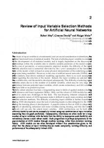
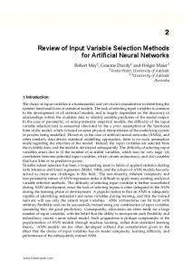
district is predominantly rural but also includes urban areas such as Bristol, Exeter, Plymouth, Torquay, Bournemouth, and Poole. Figure 1 presents the locations of 20 catchments in southwest England, and Figure 2 shows a typical catchment with the station number of 48006. The locations of catchment areas are shown in the first map together with their station numbers (the number is used to retrieve the flow records stored at the Centre for Ecology and Hydrology, United Kingdom). The areas of these catchments vary from 13.3 to 137.9 km2. 3.2. Data Source [24] The stream networks are digitized from a 1:50,000 scale topographic map obtained from the Environment Agency (EA) whereas digital elevation model (DEM) contour data (from OS Land‐Form Panorama with 10 m vertical intervals) are acquired from the EDINA service‐DIGIMAP (free maps for academic applications available at http:// edina.ac.uk/digimap/). Corine Land Cover 2000 (CLC2000) is an updated land cover database of Europe for the year of 2000 managed by the Joint Research Centre (JRC) and the European Environment Agency (EEA) where the image was taken using the Landsat 7 Enhanced Thematic Mapper (ETM). A detail explanation about CLC 2000 can be found at http://www.eea.europa.eu/. This map is used to provide land cover types in the study areas. The European Soil Data Centre (ESDAC; http://eusoils.jrc.ec.europa.eu/library/ esdac/esdac.html) is a thematic center for soil related data in Europe. ESDAC has provided a 1 km × 1 km soil raster database derived from the European Soil Database (ESDB) version 2. The 5 km × 5 km gridded annual rainfall intensity map 1961–1990 is taken from the Meteorological Office, United Kingdom (http://www.metoffice.gov.uk/), and finally, the observed Qmed values (the median annual maximum flow) for the catchments are obtained from the Environment Agency’s HiFlows‐UK Web site (http://www. environment‐agency.gov.uk/hiflows/91727.aspx). Similar data and maps used in this study should be obtainable for other parts of the world through various search engines.

4. Result [25] There are 22 catchment characteristics derived using the GIS tools from 20 catchments in southwest England. These are catchment area, longest flow path, basin length, basin perimeter, form factor, average slope, maximum relief, relief ratio, drainage density, stream frequency, bifurcation ratio, length of overland flow, land use (agriculture), land use (forest), land use (residential), land use (water and wetland), soil type (coarse), soil type (medium), soil type (medium fine), soil type (fine), soil type (peat soil) and rainfall (detailed explanations of these variables are given in section 4.1). This means there are 22 possible input variables and one output variable (i.e., the median annual maximum flow, Qmed (m3/s)) in the 20 data sets for developing the nonlinear equation for flood regionalization. 4.1. Catchment Characteristics Derivation [26] Catchment characteristics are numerical indices describing factors that influence flow regimes, and typically include measures of catchment geomorphology, soil, cli-

5 of 18

W07503

WAN JAAFAR ET AL.: VARIABLE SELECTION FLOOD REGIONALIZATION

W07503

Figure 1. Locations of 20 catchments, indicated by catchment station number, in southwest England. matology, and land use properties. The FEH contains catchment descriptors for England, where 22 catchment descriptors were derived on the basis of the catchment boundary, landform, attenuation effect due to reservoir and lake, climate, soil, and land use data. The Centre for Ecology and Hydrology [CEH, 1999] has developed a modified digital terrain model (IHDTM) from digitally held rivers and contours taken from the Ordinance Survey 1:50 000 map, so that the calculation of catchment characteristics is done using gridded elevation data. IHDTM derives catchment boundary automatically by including a 50 m × 50 m grid of drainage path directions based on the steepest route to neighboring grid nodes [Morris and Heerdegen, 1988]. This boundary can be applied to compute catchment characteristics. [27] From the aforementioned reasons, this study explores alternative catchment characteristics that are based on easily obtainable data and mostly downloadable from the Internet. The ArcGIS and ArcHydro tools are used to derive 22 catchment characteristics consisting of physical, morphological, climatological, soil type, and land use features for the 20 catchments. Table 1 provides the definitions of those catchment characteristics, and Table 2 presents the summary statistics of the calculated catchment characteristics. 4.2. Variable Selection Using the Gamma Test [28] With the GT, the input variable selection can be carried out without estimating the model parameters. A backward approach is adopted here so that the gamma test will start with all the potential input variables and gradually one variable by turn is removed by iteration. After removing

one variable, the gamma statistics are computed and this process is repeated until one variable is left. A combination that gives the lowest of the gamma value indicates the best input combination.

Figure 2. Example of a catchment from station number of 48006.

6 of 18

W07503

W07503

WAN JAAFAR ET AL.: VARIABLE SELECTION FLOOD REGIONALIZATION

Table 1. Definition of Catchment Characteristics Catchment Characteristic

Definition 2

Area (x1) Longest flow path (x2) Basin length (x3)

Area of the catchment (km ) Longest flow line in drainage basin (km) Horizontal distance along the longest dimension of the basin parallel to the main streamline Total length of the drainage basin boundary (km) Ratio between catchment area (A) and the square of basin length (BL2) Contour length (L) multiplied with its interval (I), divided by the catchment area (A), and then multiplied by 100 (%) Difference of elevation between the highest and lowest point of catchment (km) Height‐length ratio between the maximum relief (MR) and the basin length (BL) Total length of streams (∑Lt) divided by area of the catchment (A) (km/km2) Ratio between the total number of stream segments of all orders (∑Nu) in a basin and the basin area (A) Number of streams of a given order (Nu) to the number of segments of the higher order (Nu + 1) One half of the reciprocal of the drainage density (km) Agriculture area (%) Forest area (%) Residential area (%) Water bodies and wetland (%) Soil type consists of 65% sand (%) Soil type consists of 18% –35% clay and ≥15% sand or