Bézier Parameterization for Optimal Control by Differential ... - CiteSeerX

Bézier Parameterization for Optimal Control by Differential Evolution T. Rogalsky Mathematics, Canadian Mennonite University, Winnipeg, Manitoba, Canada

Abstract - Direct solution methods for optimal control problems treat them from the perspective of global optimization: perform a global search for the control function that optimizes the required objective. Increasingly, Differential Evolution is being recognized as a powerful global optimizer for optimal control. A parameterization technique is required, which can represent control functions using a small number of real-valued parameters. Typically, direct methods using Differential Evolution parameterize control functions with a piecewise constant approximation. In this paper a new parameterization is introduced, using Bézier curves, and is combined with Differential Evolution into a new evolutionary direct method for optimal control. The effectiveness of the new method is demonstrated by solving a range of optimal control problems. Keywords: Control Vector Parameterization, Differential Equations, Evolutionary Algorithms, Optimal Control

1

Introduction

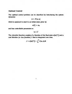
In many mathematical models, the dynamics are described by a system of ordinary differential equations for a set of dependent functions, x(t). When these systems are also controlled by a second set of independent functions, u(t), an obvious goal is to find u(t) that optimizes, in some sense, the dynamical system. This type of problem is known as optimal control, or sometimes, dynamic optimization. Mathematically, the problem can be stated as follows: tf

min F (u ) = u

∫ f (t , x(t ), u(t )) dt , t0

x′(t ) = g (t , x(t ), u(t )) subject to  , x (t0 ) = x 0

(1)

where t 0 and t f are the initial and final times, and f and g depend on the particular model. The dependent functions x(t) are known as state functions, and the independent u(t) as control functions. For example, in a model of an epidemic disease, the state functions might be the populations, at time t, of those who are susceptible to the disease, those who are immune from the

disease, and those who are recovered from the disease. Control functions might include a vaccination rate and a quarantine rate, both functions of time. One possible goal would then be to find a public health policy represented by control functions that minimize both the number of infectious persons, and the cost of implementing the policy. There are two general approaches to optimal control. These are often labeled as direct and indirect methods. An indirect method transforms the problem into a boundary value problem (BVP), which can then be solved analytically or numerically using well-known techniques for differential equations. An excellent introduction to this method can be found in a recent text by Suzanne Lenhart and John Workman [1]. In a direct method, optimal control is seen as a standard optimization problem: perform a search for the control function u(t) that optimizes the objective functional. Evolutionary algorithms, such as Differential Evolution (DE) [2], are powerful global optimizers, but they do not operate on infinitedimensional spaces. So before optimizing, a parameterization method is required, whereby the functions of continuous time can be approximated by a discrete set of parameters. Typically, direct methods using DE simply discretize the control function space. That is, control functions are approximated using a piecewise constant parameterization. When the optimal solution is continuous, then, one must choose between accuracy and efficiency. A large number of parameters will converge slowly to an accurate approximation of the true solution, while a small number will converge quickly to a poor approximation. In this paper, a new direct method is developed for optimal control, using DE in conjunction with Bézier curves to parameterize the control functions. The new method is designed to be both accurate and efficient simultaneously. Part 2 of the paper examines evolutionary direct methods in general. In Part 3 the Bézier parameterization is developed for use with DE. Part 4 applies the method to several optimal control problems. The focus here is to confirm that this new direct method is effective and efficient for a broad range of problems. In each case, the examples used can be solved analytically by an indirect method. This permits comparison of the two solutions, and validates the method. Finally, Part 5 looks ahead to future implementations and applications.

2 2.1

Direct methods for optimal control Direct vs. indirect methods

There are certain mathematical advantages to using an indirect method, including existence and uniqueness results, exact solutions when the BVP can be solved analytically, and error estimates when it is solved numerically [1]. There are also several limitations which can be overcome by a direct method. First among the limitations of an indirect method is that each solution is problem-specific. A separate mathematical transformation must be derived for each distinct optimal control problem, and in some cases the mathematics can be rather complicated. A direct method, on the other hand, is a more universal solution, which can be easily and quickly applied to a new control problem. Second, in an indirect method, the transformation requires that the optimal control problem be formulated with a single objective functional. When there are multiple objectives, they must be collected into one. By contrast, direct evolutionary methods can use a multiobjective global optimizer. One numerical run can produce a range of solutions that can be considered mutually optimal in some sense [3]. Third, applied optimal control problems often have multiple, complicated constraints. In the indirect method, these are be difficult to impose, and can lead to intractability [4n]. In a direct evolutionary method, constraints are easily imposed with a penalty function. Examples are given below. Fourth, because the indirect method relies on variational calculus, it is of necessity a local optimization method. But complicated systems sometimes have multimodal landscapes with many local optima. In these cases, a global, evolutionary optimization scheme can be more effective [5].

2.2

Evolutionary direct methods

Evolutionary Algorithms (EAs) are powerful, global optimizers, that treat optimization from the perspective of natural evolution: an initial population of feasible solutions evolves into a population of globally near-optimal solutions. There are typically two mechanisms by which new feasible solutions are formed: mutation (small perturbations in a binaryor real-valued individual) and recombination (combining the characteristics of two different individuals). Some form of natural selection is used to decide which population members “survive” to the next generation, and after many generations the population converges, to one or several near-optimal solutions. There are two types of EA, distinguished by the way in which they represent individual feasible solutions. Genetic Algorithms (GAs) [6] use binary representation, and are thus suitable for discrete or integer optimization problems. Evolutionary Strategies (ESs) [7] use real-valued vectors, and are better suited for the kind of continuous parameter optimization required for optimal control. DE emerged in the 1990s as one of the most impressive ESs, converging faster and with more certainty than many other acclaimed global optimization methods [3]. In the years since, it has successfully been used in many different applied fields

[2]. DE has been shown to be a robust and efficient global optimizer for an evolutionary direct approach – in a variety of specific applications [8]-[11], and more generally for optimal control problems that have multimodal control function landscapes [5].

2.3

Control Vector Parameterization

To use an ES for optimal control, a parameterization strategy is required by which control functions can be represented by the Rn vectors on which DE operates. This is known as Control Vector Parameterization (CVP). A wide variety of CVPs have been used with non-evolutionary optimizers, including piecewise constant [12], Chebyshev polynomials [13], Lagrange polynomials [14], and piecewise Lagrange polynomials [15]. Direct methods using DE have been less creative, relying almost exclusively on piecewise constant CVP. Each DE-based solution referenced above [5], [8]-[11] approximates the control as a piecewise constant function. The reason may be that it is the easiest parameterization to encode, or it may be that current researchers are simply following the path trod by those who first applied EAs to optimal control [16], [17]. In any case, there is room for improvement. The limitations of a piecewise constant approximation are obvious: a very high number of parameters is needed for an accurate approximation. However, EAs are computationally expensive, and require a small number of parameters to converge to a near-optimal solution within a reasonable amount of time. Thus, a more creative CVP is desirable for evolutionary direct methods. To be effective, the CVP should be able closely to approximate arbitrary, continuous, control functions. To be efficient, it must do so with a relatively small number of parameters. Also, CVPs that increase the nonlinearity of the objective function can lead to epistasis [18] – the nonlinear and interdependent manner in which the objective function relates to the design parameters. Small changes in several variables can result in large changes in the objective function. Epistatic functions can lead to premature convergence, because they provide so few clues as to the location of the global minimum. In general, a reduction of this nonlinear interaction, by having parameters more directly linked to the objective function, will enable the optimizer to converge more quickly.

3 3.1

Bézier parameterization for Differential Evolution Bézier Control Parameterization

P. Bézier, of the French firm Regie Renault, pioneered the use of computer modeling of surfaces in automobile design. His UNISURF system, initiated in 1962 and used by designers since 1972, has been applied to define the outer panels of several cars marketed by Renault [19], [20]. The foundations of Bézier curves, however, go back much further. In 1926, S. Bernstein presented a constructive proof of the Weierstrass approximation theorem [21], using functions that have become

known as Bernstein polynomials. Bézier curves have a very similar form, and are sometimes referred to as Bézier-Bernstein polynomials. Bézier curve parameterization is used regularly in engineering applications, such as shape optimization. It has been used effectively with DE to optimize turbomachinery airfoils [22]. An extensive search of the literature, however, suggests that this is the first use of a Bézier CVP for optimal control by any direct method, whether evolutionary or nonevolutionary. An nth order Bézier curve, P(z), is defined parametrically using n+1 two-dimensional control points Pi (ti , ui ) , as follows: n

P( z ) =

n!

∑ P i !(n − i )! z (1 − z ) i

i

n −i

, 0 ≤ z ≤ 1,

(2)

i=0

where z is the parameter. Bézier curves begin at control point P0, end at control point Pn, have initial slope equal to that of the line segment P0P1, ending slope equal to that of Pn-1Pn, and always lie within the convex hull formed by the control points. The curve is nth order continuous throughout and never oscillates wildly away from its defining control points. Thus Bézier curves can parameterize smooth, non-oscillatory functions, with minimal epistasis, using only a few parameters. The Bézier Control Parameterization (BCP) introduced here is designed for a single control function. A fixed, regular mesh is used on the t-axis. This forces the curve to be singlevalued, and also reduces the dimension of the optimization vectors to n+1. That is, the BCP u = [ ui ]i = 0 completely n

encodes a control function u(t) as the nth order parametric Bézier curve u (t ) = t ( z ), u ( z ) , as follows:

n! t ( z ) = n t + i∆t i n −i  z (1 − z ) ) ∑( 0   i !( n − i )! i =0   , 0 ≤ z ≤ 1, (3) n n! i n −i u ( z ) = ∑ u  z (1 − z ) i i !( n − i )!   i=0 where ∆t = (t f − t 0 ) / n , t 0 is the initial time, and t f is the final time. The objective function, F(u), is computed as follows. The control function u(t), is found using the Bézier curve parameterization. It is stored as a set of data points, at parameters z=0,h,2h,…,1. A step-size of h=0.01 is used here, and can be refined when more accuracy is required. The IVP is then solved numerically for x(t), interpolating the data points to approximate u(t) as necessary. The differential equation solver used is MATLAB’s ode45 function, an explicit Runge-Kutta (4,5) formula, with the Dormand-Prince pair. Finally, the objective integral is evaluated, again interpolating to approximate x(t) and u(t), as necessary. The numerical integration routine is MATLAB’s quad function, a recursive adaptive Simpson quadrature. The value of the integral is the “cost” F of the vector u.

3.2

Differential Evolution Optimization of the function F(u) is performed using DE,

which minimizes the cost of a population of vectors u. The crucial difference between DE and other ESs lies in mutation. ESs normally use predetermined probability distribution functions to perturb vectors, leaving them unable to adapt the perturbation magnitude to the topology of the objective function. DE uses the “differential” of two randomly chosen population vectors, ua and ub, to perturb a base vector uc, u new = u c + F ( u a − u b ) , where F is the differential weight. The perturbation magnitude is thus automatically appropriate to the given landscape, and the search is less random, being dictated by the shape of the objective function itself. This property of DE is known as self-organization. Ultimately, it results in better convergence properties as the algorithm nears the global minimum. Two DE strategies are used here. In DE/local-to-best/1, the base vector is a combination of one randomly chosen vector and the vector with the lowest objective function value. F=0.85 is the recommended differential weight. This strategy tends to balance robustness with fast convergence, and has been demonstrated as one of the more effective DE strategies [23]. Usually a population size of NP=10D is effective, where D=n+1 is the dimension of the vector u. Occasionally, when misconvergence occurs, NP needs to be increased. For small population sizes, a fast convergence strategy is DE/best/1 with jitter. Here the base vector is the best one in the population, which tends to reduce robustness. When the problem dimension and the population size are small, this loss can be balanced by jittering, the practice of generating a different value of F for each parameter. This results in small, random variations in both scale and orientation of the differential [2].

4

Results

Below we consider several representative problems from [1]. The purpose here is to demonstrate that the DE/BCP direct method can find accurate solutions to the standard range of optimal control problems. Thus, in addition to one problem in standard form, also considered are examples with payoff terms, with fixed state endpoints, and with bounded controls. Both minimization and maximization problems are considered. Most have a single state function, but for completeness the final example has multiple state functions. Each test case has a single control function, but the method can be extended to solve problems with multiple controls. All problems considered have continuous optimal controls, and can be solved analytically. This allows validation of the BCP, by comparing its result with the exact solution. Details of the exact solutions can be found in [1].

4.1

Standard form

The standard form for optimal control problems is (1). In the following example, there is one control function u(t), and one state function x(t):

1

min F (u ) = u

∫ ( 3 x (t )

2

)

min F (u ) =

+ u (t ) dt , 2

u

0

(4)

 x ′( t ) = x ( t ) + u ( t ) subject to  .  x (0) = 1 3e

−4

3e

e − 2t

−4

3e + 1

x (t ) =

−4

3 −4

3e + 1 1

e

−2 t

.

(5)

−2 t

e + −4 e −4 3e + 1 3e + 1 The BCP solution has n=3, representing four Bézier control points. DE parameters are DE/best/1/jitter, F=0.85, CR=1, with population size NP=15. The initial population is formed by random selection of control parameters, within the bounds [-3,0]. Optimization is terminated after 50 generations. The jitter strategy, in this case, was very effective, converging to an excellent solution in under two minutes, using a current Intel system. The control points for the BCP solution are shown in Table 1. 2t

Table1. BCP solutions to optimal control problems of part 4. The Bézier curve control function is defined by (3) for unconstrained problems; and (3) and (11) for constrained problems. Optimal Degree Bézier Control Parameterization control n u0 u1 u2 u3 problem (4) 3 -2.7774 -0.9353 -0.5457 0.0043 (7) 3 -2.0017 -1.3363 -0.9849 -0.7331 (9) 3 -0.7052 -0.5110 0.6082 1.2481 (12) 2 4.7188 -1.5990 -0.8749 (13) 2 14.726 -0.1696 0.7300 (15) 2 3.0036 1.4924 0.0044

4.2

Payoff term

In some optimal control problems, there can be one objective over the entire time interval, and a second objective at a specific time, usually the final time tf. The first is represented by an integral, and the second by a function of the time tf. The two are typically combined into one objective functional through a weighted sum, tf

min F (u ) = u

∫

1

∫ u (t ) dt + x(1) , 2 2

2

0

f1 (t , x (t ), u (t )) dt + af 2 (t f ) ,

(6)

t0

where a is the weight of the second objective relative to the first. The term outside the integral, af 2 (t , x (t ), u (t )) , is known as a payoff term. These might be necessary when, for example, a second objective is to minimize the final population. In this test case, the integral objective depends only on the 2

control, and the payoff term, x (1) , depends only on the state:

(7)

 x ′(t ) = x (t ) + u (t ) subject to  .  x (0) = 1 −t

The analytical solution is:

u (t ) =

1

−t

The analytical solution is: u (t ) = −2e , x (t ) = e . The BCP solution has n=3. The DE strategy used is DE/best/1/jitter, F=0.85, CR=1. Population size was increased to NP=25, to improve the global convergence. The initial population is formed by random selection of control parameters, within the bounds [-5,5]. Optimization is terminated after 50 generations. The BCP solution (Table 1) once again closely approximates the actual solution.

4.3

Fixed state endpoint

In standard optimal control problems, the state equations are initial value problems. But in some cases, the state is fixed not only at its initial point, but also its endpoint. Such is the case in the third example:

min F (u ) = u

∫

4

0

u (t ) + x (t ) dt , 2

 x′(t ) = u (t ) .  x (0) = 0, x (4) = 1

(8)

subject to 

The actual solution is: optimal control u (t ) = (2t − 3) / 4 and optimal state x (t ) = (t − 3t ) / 4 . When finding the solution by an indirect method, the fixed endpoint can be included in the transformation to a BVP. However, the DE/BCP direct method uses a Runge-Kutta initial value problem solver, which cannot handle the fixed state endpoint. Thus it is necessary to reformulate the problem. One way to do this is to formulate the state equations as a constrained initial value problem, with the fixed state endpoint as the constraint. Evolutionary algorithms typically deal with constraints by using a penalty function, in which a numerical penalty is added to the objective function whenever the solution doesn’t meet the constraint. Penalties imposed are proportional to the extent to which the constraint is violated. The penalty function formulation of (8) is as follows: 2

min F (u ) = u

∫

4

0

u (t ) + x (t ) dt + µ x (4) − 1 , 2

 x ′(t ) = u (t ) ,  x (0) = 0

(9)

subject to 

where µ is a scaling constant, representing the weight of the penalty relative to the objective functional. The BCP solution to (9) has n=3. The DE strategy used is DE/best/1/jitter, F=0.85, CR=1, NP=25, terminating after 50 generations. The penalty scaling constant was µ=10. The BCP solution (Table 1) closely approximates the actual, linear solution, and has a state endpoint of x(4)=0.99996. Endpoints closer to the required value of x(4)=1 could be achieved by increasing the scaling constant.

4.4

Constrained control

In first three sample problems, the control function was unconstrained. Many models, however, required upper or lower bounds on the control. In such cases, the typical evolutionary approach to constrained optimization is to introduce a penalty function. For example, if uUB (t ) is an upper bound on control function ui (t ) , one could add an integral penalty to the

For this problem, it is sufficient to use three Bézier control points for an excellent solution. However, both the population size and maximum number of generations had to be increased to find a global solution. This resulted in the DE/best/1/jitter strategy being rather inefficient. A better result was obtained with DE/local-to-best/1, NP=40, F=0.85, CR=1, and 100 generations. An excellent solution is obtained, shown in Fig. 1, with BCP solution given in Table 1.

objective function:

optimal control 6

tf

u

∫ f (t , x(t ), u(t )) dt + µ ∫ ( u (t ) − u i

1

UB

(t ) ) dt . (10)

BCP solution 4

control points

ui ≥ uUB

t0

This approach is inadequate for the BCP method, because the solutions to constrained control problems are often nondifferentiable. Bézier curves, on the other hand, are not only differentiable, but smooth, having continuous derivatives of all orders. An alternate approach is simply to redefine the control, piecewise, to equal the constraint whenever the Bézier curve violates it. That is, the BCP method computes the Bézier curve, u Bez (t ) , as usual from (3), but the control function itself is

u Bez (t ), u LB ≤ u Bez (t ) ≤ uUB  u (t ) = u LB , u Bez (t ) < u LB , u , u (t ) > u  UB Bez UB

actual solution 2 0 -2 0

0.5

u

2

0

actual solution

40

0

(12)

such that 0 ≤ u (t ) ≤ 2. Note that while DE solves minimization problems, (12) is a maximization problem. It is converted to the dual problem by minimizing − F (u ) . The actual solution is defined piecewise on three intervals, and I1 = [ 0, 2 − ln(4.5) ) , I 2 = [ 2 − ln(4.5), 2 − ln(2.5) ] , I 3 = ( 2 − ln(2.5), 2 ] , with:

t ∈ I1  2,  2 −t u (t ) = e − 5 2, t ∈ I 2 , and 0, t ∈ I3  7e t − 2, t ∈ I1  −2 t 2 −t x (t ) = ( 7 − 81e 8 ) e − e 2 + 5 2 , t ∈ I 2 .  −2 t t ∈ I3 ( 7 − 7e ) e ,

2

BCP solution

0

2

 x′(t ) = x (t ) + u (t ) ,  x (0) = 5

1.5

optimal state

20

2 x (t ) − 3u (t ) − u (t ) dt ,

subject to 

2

(11)

or constant. In the following example, the control is bounded from above and below:

∫

1.5

60

0.5

where upper and lower bounds, uUB and u LB , can be functions

max F (u ) =

1 t

x(t)

defined as

u(t)

min F (u ) =

1 t

Fig. 1. Solutions of (12), an optimal control problem with constraints on the control. The BCP solution found by DE is compared to the actual, analytic solution. Our experience generally with DE has led us to conclude that the strategy DE/local-to-best/1 is effective for a wide variety of problems, nicely balancing robustness with fast convergence. Normally a population size of NP=10D works well, but in this case, where dimension was D=3, NP had to be increased slightly to 40. In practice, when the actual solution is unknown, the results of several population sizes should be compared, to ensure a global solution.

4.5

Constrained control with payoff

In this example, we demonstrate a BCP solution for a problem with mixed constraints, both an upper bound on the control and a payoff term for the state: 4

max F (u ) = x (4) − ∫ u (t ) dt , u

subject to

2

0

 x ′( t ) = x ( t ) + u ( t ) ,   x (0) = 0

such that u (t ) ≤ 5. The actual solution has optimal control and state: 0 ≤ t < 4 − ln(10) 5, u (t ) =  4 − t , e 2 , 4 − ln(10) ≤ t ≤ 4

(13)

incorporated into the objective function with a penalty formulation, so that the problem is reformulated as follows:

0 ≤ t < 4 − ln(10) 5e t − 5, . x (t ) =  4 − t −4 t  − e 4 + ( 5 − 25e ) e , 4 − ln(10) ≤ t ≤ 4

min F (u ) =

The BCP solution uses three Bézier points, with DE strategy DE/local-to-best/1, NP=40, F=0.85, CR=1, and 100 generations. The result is a BCP solution (Table 1) closely approximating the actual solution (Fig. 2).

BCP solution

u(t)

subject to

1

0

x2 (t ) + u (t ) dt + µ x1 (1) − 1 , 2

 x1′ (t ) = x2 (t ), x1 (0) = 0 .   x2′ (t ) = u (t ), x2 (0) = 0

(15)

Three Bézier control points are used in the solution, with DE strategy DE/local-to-best/1, NP=25, F=0.85, CR=1, and 50 generations. The penalty scaling constant is µ = 10 . The BCP solution (Table 1) is again in excellent agreement with the actual solution (Fig. 3).

optimal control 15 10

u

∫

control points actual solution

5

optimal control

0

4 BCP solution

-5 0.5

1

1.5

2 t

2.5

3

3.5

3

4 u(t)

0

optimal state

control points actual solution

2

300 1

BCP solution actual solution

200

0

x(t)

0

0.2

0.4

0.6

0.8

1

0.8

1

t 100

optimal state 2 BCP solution

0 0.5

1

1.5

2 t

2.5

3

3.5

1.5

4 x(t)

0

Fig. 2. Solutions of (13), an optimal control problem with mixed constraints. The BCP solution found by DE is compared to the actual, analytic solution.

4.6

subject to

∫

1

0

x2 x1

0 0

0.2

0.4

0.6 t

All of the above examples have been for optimal control of a single differential equation in one state variable. The extension of the BCP/DE solution method to a system of differential equations is essentially trivial. The Runge-Kutta solver, used to solve one equation in the previous test cases, is designed for any number of differential equations. Thus no additional code is required when there are multiple state functions, as long as there remains only one control function. For the sake of completeness, however, we demonstrate the ability of the BCP/DE technique to solve an optimal control problem with multiple state variables. In the following problem, there are two state variables, one of which has fixed initial and ending point: u

1 0.5

Multivariable optimal control

min F (u ) =

actual solution

x2 (t ) + u (t ) dt , 2

 x1′ (t ) = x2 (t ), x1 (0) = 0, x1 (1) = 1 (14) .   x2′ (t ) = u (t ), x2 (0) = 0

The actual solution is u (t ) = 3 − 3t , x1 (t ) = 3t 2 − t 2 , 2

3

x2 (t ) = 3t − 3t 2 . 2

As above, the fixed endpoint for the first state variable is

Fig. 3. Solutions of (15), an optimal control problem with multiple state functions. The BCP solution found by DE is compared to the actual, analytic solution.

5

Conclusions

The BCP method proves successful for each optimal control problem, producing an accurate approximation of the true solution, using a small number of parameters. For evolutionary direct methods, it provides a means to improve both accuracy of the final result and efficiency of the algorithm. It has been demonstrated that the technique is effective for all classes of optimal control problems. The direct method developed here has potential to be a simple, general solution method for any optimal control problem. This can be extremely helpful in the field of epidemiological and biomedical modeling, in which researchers requiring an optimal public health policy or optimal treatment schedule may not have the mathematical skills, or the time, to solve the model indirectly. In other work, we intend to demonstrate the efficacy of the BCP method for these types of models. Many of these have multiple control functions, e.g. vaccination rate, quarantine rate, and isolation rate for an

epidemic. Thus the method will have to be extended to allow for multiple controls. The true value of a direct evolutionary method, of course, is not to reproduce known solutions to optimal control problems, but to provide an alternate solution method for problems that are difficult or impossible to solve indirectly. Having validated the method generally, it is to these that attention can now be turned, particularly problems that are multiobjective, that are multimodal, and that have complicated constraints.

Acknowledgment The author thanks Dr. Abba Gumel, professor of mathematics at University of Manitoba, for suggesting the problem of optimal control, motivated by his work in epidemiological modeling.

References [1] Suzanne Lenhart and John T. Workman, Optimal Control Applied to Biological Models. Boca Raton: Chapman & Hall/CRC, Taylor & Francis Group, 2007. [2] Ken Price, Rainer Storn, and Jouni Lampinen, Differential Evolution: A Practical Approach to Global Optimization. New York: Springer, 2005. [3] Kalyanmov Deb, Multi-Objective Optimization Using Evolutionary Algorithms. New York: John Wiley & Sons, 2001. [4] John McCall, “Genetic algorithms for modelling and optimization,” Journal of Computational and Applied Mathematics, vol. 184, no. 1, pp. 205-222, Dec. 2005. [5] I.L. Lopez-Cruz, L.G. Van Willigenburg, and G. Van Straten, “Efficient differential evolution algorithms for multimodal optimal control problems,” Applied Soft Computing, vol. 3, no. 2, pp. 97–122, Sept. 2003. [6] D.E. Goldberg, Genetic Algorithms in Search, Optimization, and Machine Learning. Reading: AddisonWesley, 1989. [7] Hans-Georg Beyer: The Theory of Evolution Strategies. New York: Springer, 2001. [8] J.P. Chiou and F.S. Wang. "A hybrid method of differential evolution with application to optimal control problems of a bioprocess system," Proc. IEEE International Conference on Evolutionary Computations, IEEE World Congress on Computational Intelligence, New York, 1998, pp. 627–632. [9] M.H. Lee, Ch. Han, and K.S. Chang, “Dynamic optimization of continuous polymer reactor using a modified differential evolution algorithm,” Ind. Eng. Chem. Res., vol. 38, no. 12, pp. 4825–4831, Dec. 1999. [10] I.L. Lopez-Cruz, L.G. van Willigenburg, and G. van Straten. “Optimal control of nitrate in lettuce by a hybrid approach: differential evolution and adjustable control weight

gradient algorithms,” Computers and Electronics Agriculture, vol. 40, nos. 1-3, pp. 179-197, Oct. 2003.

in

[11] M.D. Kapadi and R.D. Gudi, “Optimal control of fedbatch fermentation involving multiple feeds using differential evolution,” Process Biochemistry, vol. 39, no. 11, pp. 1709– 1721, July, 2004. [12] C.J. Goh, K.L. Teo, “Control parametrization: a unified approach to optimal control problems with general constraints,” Automatica, vol. 24, no. 1, pp. 3–18, Jan. 1988. [13] J. Vlassenbroeck, “A chebyshev polynomial method for optimal control with state constraints,” Automatica, vol. 24, no. 4, pp. 499–506, July 1988. [14] L. Biegler, “Solution of dynamic optimization problems by successive quadratic programming and orthogonal collocation,” Comp. Chem. Engng., vol. 8, nos. 3-4, pp. 243– 248, 1984. [15] V.S. Vassiliadis, R.W.H. Sargent, and C.C. Pantelides, “Solution of a class of multistage dynamic optimization problems 1. Problems without path constraints,” I&EC Res., vol. 33, no. 9, pp. 2111–2122, Sept. 1994. [16] S. Smith, “An Evolutionary Program for a class of continuous optimal control problems,” Proc. IEEE Conference on Evolutionary Computation, vol. 1, Piscataway, pp. 418– 422, 1995. [17] N.V. Dakev, A.J. Chipperfield, and P.J. Flemming, “A general approach for solving optimal control problems using optimization techniques,” Proc. IEEE Conference on Systems, Man and Cybernetics, part 5, Vancouver, pp. 4503–4508, 1995. [18] Bäck, Thomas Evolutionary Algorithms in Theory and Practice: Evolution Strategies, Evolutionary Programming, Genetic Algorithms. New York: Oxford University Press, 1996. [19] P. Bézier, Numerical Control – Mathematics and Applications, translated by A.R. Forrest and A.F. Pankhurst, London: John Wiley & Sons, 1972. [20] P. Bézier, "Mathematical and Practical Possibilities of UNISURF," in Computer-Aided Geometric Design, R.E. Barnhill and R.F. Riesenfeld, Eds. New York: Academic Press, 1974, pp. 127-152. [21] P.J. Davis, Interpolation and Approximation. New York: Blaisdell Publishing Company, 1963. [22] T. Rogalsky, R.W. Derksen, and S. Kocabiyik, “Differential Evolution in Aerodynamic Optimization,” Canadian Aeronautics and Space Journal, vol. 46, no. 4, pp. 183-190, Dec. 2000. [23] A. Auger, N. Hansen, J.M. Perez Zerpa, R. Ros, M. Schoenauer. “Experimental Comparisons of Derivative Free Optimization Algorithms” in Lecture Notes in Computer Science, Vol. 5526: Proceedings of the 8th International Symposium on Experimental Algorithms, pp. 3-15. New York: Springer-Verlag, 2009.