Sep 2, 2011 - Ricardo de Castro, Rui Araujo, Diamantino Freitas. Faculdade de Engenharia da Universidade do Porto,. Portugal, (e-mail: {de.castro, raraujo, ...
Preprints of the 18th IFAC World Congress Milano (Italy) August 28 - September 2, 2011
Optimal Linear Parameterization for On-Line Estimation of Tire-Road Friction Ricardo de Castro, Rui Araujo, Diamantino Freitas Faculdade de Engenharia da Universidade do Porto, Portugal, (e-mail: {de.castro, raraujo, dfreitas}@fe.up.pt) Abstract: In this article, we propose a linear parameterization (LP) for representing the friction in the tire-road interface, suitable for on-line identification. This model was obtained by employing function approximation techniques, which results in an optimization problem to minimize the fitting error between the LP and the nonlinear Burckhardt model. Compared with others LPs proposed in the literature, the optimal LP features a reduced number of parameters and good approximation capabilities. Moreover, the proposed model can be identified though linear identification techniques, simplifying the on-line peak friction estimation. Simulation results obtained with a vehicle simulator demonstrates the effectiveness of the proposed parameterization. Keywords: Tyres, Friction, Function approximation, Parameter estimation 1. INTRODUCTION
In automotive applications, the adhesion conditions present in the tire-road interface have a strong influence in the tire ability to generate longitudinal and lateral forces and, under reduced grip conditions, represent a potential menace to the vehicle safety. With the recent proliferation of active safety systems (like ABS, TCS, ESP and VDC) (van Zanten, 2002), the estimation of adhesion levels, characterized by the friction coefficient, has attracted a growing interest in the research community, since the knowledge of this variable contributes significantly to increase the effectiveness of these safety systems. Unlike other easily measurable variables, such as the vehicle acceleration, yaw rate and wheel speeds, currently, there is no economically viable sensor that can be installed in the vehicle to measure the friction coefficient. These difficulties have encouraged the development of virtual sensors to estimate this variable using easily measurable signals. There are several approaches to tackle the friction estimation problem. In this article we focus on the so-called slip-based techniques, i.e. use tire force models based on the wheel slip to infer the adhesion levels (Rajamani et al., 2010), and constrained our study to the friction estimators active during longitudinal vehicle manoeuvres. These methods can be divided in two categories: qualitative and quantitative (see Figure 1). In both cases, the main objective is to obtain an estimation of the peak friction coefficient, but the output of the two mentioned methods is very different. In the first case, qualitative, the output of the estimator is based on a grading system, providing an indicator of adhesion quality, for instance qualifying the grip levels in a scale from ’A’ (high grip) to ’E’ (very slippery); in the second case, quantitative, a numeric output is generated to quantify with more detail the adhesion. Copyright by the International Federation of Automatic Control (IFAC)
Examples of the qualitative approach can be found on references (Gustafsson, 1997; Ono et al., 2003; Muller et al., 2003; Wang et al., 2004; Rajamani et al., 2010). The main driving force behind these approaches is the problem of persistence of excitation: in order to extract the peak friction we need to apply high levels of tire slip, which is not desirable from the safety point of view. To avoid this problem, the qualitative methods identify the tire longitudinal stiffness, i.e. the friction slop for low slip values, and, then, infer the grip levels through a classification process that correlate the slop value with the peak friction (see Figure 1). Albeit these approaches solve the problem of persistence of excitation, they also introduce a new issue: the classification stage. This classification is very problematic to obtain in practice and, as pointed out by (Gustafsson, 1997) and (Carlson and Gerdes, 2005), varies with the type of tires, tire wear, pressure and temperature, among many other factors. Therefore, a significant experimental effort is required to tune the classification process, which makes these qualitative approaches very difficult to apply in practice. On the other hand, the quantitative methods (Kiencke, 1993; Germann et al., 1994; Kiencke and Nielsen, 2005; Yi et al., 2002; Tanelli et al., 2009; Yi et al., 2002), extract the peak friction using only on-line curve fitting techniques. Although the estimation is obtained at expense of applying high tire slips, the estimation process is more simple and robust and also offers the possibility to identify the optimal slip reference λmax associated with the maximum friction point. This last feature is very useful to generate the reference signal used in some anti-lock braking and traction control systems that relies on wheel slip control (Tanelli et al., 2009; Hori, 2004). Furthermore, since the most common tire models, like the Magic Tire Formula (Pacejka, 2002) or the Burckhardt representation (Kiencke and Nielsen, 2005), are nonlinear, the online identification of the model parameters tend to be very
8409
Preprints of the 18th IFAC World Congress Milano (Italy) August 28 - September 2, 2011
Peak Detector
Regression m
^
Fx ^ Fz v^ rw^
(l, m) Calculation m =
Fx Fz
l=
v - rw v
^ m(l,q)
The most common approach to represent the friction coefficient µ(.) is based on the static Burckhardt (Kiencke and Nielsen, 2005) model:
^ max m
^ max m
^l max
^lmax
l
µ(λ, β) = β1 (1 − e−β2 λ ) − β3 λ and the magic tire formula (MTF) (Pacejka, 2002):
Quantitative Method
l,m
(3)
Classification
Regression m
q
^ max m
A B C D E
µ(λ, β) = β1 sin (β2 atan((1 − β4 )β3 λ + β4 atan(β3 λ))) (4) where the vector β = [β1 β2 ... βd ]T represents the model parameters.
q
l
Qualitative Method
Figure 1. Estimation methods for detecting the longitudinal peak friction.
3. OPTIMAL LINER PARAMETERIZATION
difficult. As a result, most of the quantitative method uses linear parameterizations (LP), i.e. nonlinear models whose unknown parameters can be identified by linear techniques.
In this section we will present the derivation of an optimal LP, in the sense that it provides the best fit of a nonlinear friction model over a given parametric region of interest, as described in the next problem: Problem 1. (Linear Approximation of µ) Consider a given parametric model f (λ, β), typically nonlinear (such as (3) or (4))
In this article we offer a contribution to the quantitative methods, by proposing a more rational approach to derive the LP. Unlike the before mentioned parameterizations, which are build using heuristics considerations, we employed function approximation techniques to find and equivalent, but linear identifiable, model to the nonlinear Burckhardt representation. The resulting LP yields a more accurate approximation and, in some cases, requires less number of parameters, which gives some practical advantages for on-line friction identification.
f: S ×P →R (5) which describes the friction coefficient curve in the domain (λ, β) ∈ S × P ⊂ [0, 1] × Rd . The slip variable λ is the model input and the β vector contains the model internal parameters, which are unknown and possibly time-varying. To approximate this nonlinear model consider the parameterization:
2. LONGITUDINAL VEHICLE/TIRE MODEL
� � fˆ(λ, w, θ) = h1 (λ, w) . . . hn (λ, w) θ
(6a)
T
In this section, an introduction to the models associated with friction estimation methodology is briefly discussed. Since we are considering longitudinal forces and slip, the quarter car model, widely used in the literature of the area (Tanelli et al., 2009; Kiencke and Nielsen, 2005; Canudas-de Wit et al., 2003), is a sufficient mean to conduce our studies:
= H(λ, w) θ (6b) n where {w, θ} ∈ R × R is a vector of parameters and hi (λ, w), i = 1, ..., n the basis functions.
J ω˙ = rFx − Tb
(1a)
M v˙ = −Fx
(1b)
Notice that, after solving the previous problem and finding w∗ , we can insert this vector in (6) and transform the nonlinear model into a linear parameterization (LP), i.e. the model remains nonlinear, but it’s linear in the unknown parameters θ:
where ω represents the wheel angular speed, v the longitudinal vehicle speed, Tb the braking torque applied to the wheel, Fx the friction force between tire and the road, J the wheel and transmission inertia, M the equivalent mass coupled to the wheel and r the wheel radius. For simplicity, in this work we only consider the braking manoeuvres, with v > rω, but the obtained results can be effortless modified for the acceleration case. Modeling the longitudinal friction force Fx is the main difficulty in (1). Generally, the friction force is proportional to the normal force that the wheel supports (Fz ) and depends on a nonlinear function µ(.), known as the friction coefficient, which varies with the longitudinal tire slip (λ), road adhesion conditions, tire pressure, temperature, wear, among other factors, and can be grouped in a parameter vector β ∈ Rd : Fx = Fz µ(λ, β),
λ=
v − ωr v
m
Under this setting, find the vector w∗ that minimizes the modeling error 1 between fˆ(λ, w∗ , θ) and f (λ, β), over a given domain of interest [0, λ] × D ⊂ S × P. 2
T ˜ ˜ fˆ(λ, θ) = H(λ) θ H(λ) = H(λ, w∗ ) (7) Consequently, this LP can be used to identify the friction model (and the friction peak) through simple on-line recursive methods and with reduced fitting losses. To keep the problem tractable, we assume that the number (n) and the basis functions are known beforehand (later we can evaluate the fitting performance for different number and types of basis functions).
The methodology presented in this article can be applied to various types of friction curves, but for simplicity we will use the Burckhardt parameterization as the reference model, and focus on finding a LP to the single nonlinear term in this representation: 1
(2)
a performance metric to express the notion of modeling error will be presented shortly
8410
Preprints of the 18th IFAC World Congress Milano (Italy) August 28 - September 2, 2011
f (λ, β) = e−βλ
fˆo (λ) = [h1 (λ) . . . hn (λ)] θo θo = G−1 c (13a) Z λ [G]i,j = hhi , hj i = hi (λ)hj (λ)dλ (13b)
(8)
where λ ∈ [0, λ] ⊂ R and β ∈ D = [β, β] ⊂ R. In this phase, the offset and linear gain of (3) is omitted in the LP, but will be included in the final parameterization. According to (Kiencke and Nielsen, 2005), the parameter β shows a strong dependence on the road conditions (for example dry tarmac, wet tarmac, snow, etc.) and, to represent the most common types of roads, varies between β = 4 and β = 100. Additionally, since the LP will be used to extract the friction peak, it is reasonable to assume that the LP should minimize the fitting error in the slip range 0 to λ = 0.5 (it is uncommon to have friction peaks for longitudinal slips higher than 0.5). In what follows, the solution to Problem 1 was divided in two parts. In the first part, some initial assumptions are made, like considering fixed basis functions and constant β parameters, which allow us to explore some analytical results from function approximation theory. After that, these assumptions are removed and the results extended to the more general case of adaptive basis functions. 3.1 Fixed Basis Functions Under the assumptions of fixed basis functions hi and constant parameter β, we are looking for the linear parameters θ of fˆ(λ, θ) that best fits the function f . In this article, the fitting performance is defined as integral of the square fitting error (ε), which we intent to minimize:
0
Z [c]i = hf, hi i =
λ
f (λ)hi (λ)dλ
(13c)
0
where i, j = 1, . . . , n , G ∈ Rn×n , c ∈ Rn , h, i is the L2 inner product and [.]i,j refers to the row i, column j of a given matrix. Moreover, the solution is unique if the basis functions hi are linear independent. 2
Proof: Using the fact that L2 is a Hilbert space we can apply the projection theorem to solve this minimum norm problem (see (Luenberger, 1969, Chap. 3.6) for the proof details). 3.2 Adaptive Basis Functions In the previous section, it was assumed that the basis functions hi were completely know, which is the case for � �T polynomials: HP (λ) = 1 λ λ2 . . . λn−1 . However, for adaptive basis functions, i.e. m > 0, this is not true, because these functions have additional parameters for tuning. In this article we considered two of the most common types of adaptive functions (Bishop, 2006): � �T (1) Exponentials: HE (λ, w) = ew1 λ ew2 λ . . . ewn λ h iT (2) Logistic Sigmoid: HL (λ, w) = 1+e−w11 λ−w2 . . . T
λ
Z min ε(θ) = minn
θ∈Rn
θ∈R
(f (λ) − H(λ)T θ )2 dλ | {z }
0
(9)
fˆ(λ,θ)
To simplify the notation in this section, the dependence of β in f was omitted, which is reasonable as β is assumed constant for now; similarly, the basis function hi only have a λ dependence. The previous optimization problem can be � formulated in the vector space L2 [0, λ], R] , i.e. squareintegrable functions over the interval [0, λ], making use of the L2 norm: ε(θ) = kf − fˆk2 =
where w = [w1 w2 . . . wm ] ∈ Rm is a vector of parameters. We are interested in finding the vector w that minimizes the fitting error of the LP over the domain β ∈ D. To tackle this issue, we start by defining the fitting error taking in account all the variables in the problem: Z ε(θ, β, w) = 0
θ(β, w) = G−1 (w)c(β, w) (f (λ) − fˆ(λ, θ))2 dλ
(10)
Since the vector fˆ is a linear combination of L2 vectors (cf. (6)), the optimization problem (9) can be reformulated as a minimum norm problem in the L2 space, which has a simple analytical solution, described in the next Lemma. � Lemma 1. Consider the vector space L2 [0, λ], R] , a vector f ∈ L2 and a subspace M ⊂ L2 generated by the linear combination of n basis functions hi ∈ L2 : M=
fˆ ∈ L2 : fˆ =
n X
(14)
If β and w are fixed, then we can find the vector θ that minimizes ε(θ, β, w), by direct application of Lemma 1:
[G(w)]i,j = hhi (w), hj (w)i = Z λ
0
(
2
(f (λ, β) − H(λ, w)T θ ) dλ | {z } fˆ(λ,w,θ)
λ
Z
λ
) hi θi ,
hi ∈ L2 ,
θi ∈ R (11)
hi (λ, w)hj (λ, w)dλ (15) 0
Z [c(β, w)]i = hf (β), hi (w)i =
λ
f (λ, β)hi (λ, w)dλ(16) 0
where i, j = 1, . . . , n. It should be noted that, unlike the previous section, with adaptive functions the matrix G depend on the parameter w, while the vector c depends on both w and β. Therefore, we can eliminate the dependence on θ and define the fitting error as:
i=1
Z
Then, the minimum norm problem:
ε(β, w) =
λ
2
(f (λ, β) − H(λ, w)T G−1 (w)c(β, w)) dλ
0
min kf − fˆk2
fˆ∈M
has the solution:
(12)
(17) In order to measure the performance of the LP over the parametric range of interest, i.e. D, it is convenient to
8411
Preprints of the 18th IFAC World Congress Milano (Italy) August 28 - September 2, 2011
Table 1. Total error εT for fitting (8) with different LPs.
In summary, the optimal LP for approximating (8) was found to be exponential based, with n = 4 and n = 3:
Number of basis (n) Basis Type
1
2
3
4
Polynomial (HP )
-
0.6844
0.3857
0.2127
Log. Sigmoid (HL )
0.2849
0.0467
0.0212
0.0059
Exponential (HE )
0.2870
0.0362
0.0046
0.0005
(Tanelli et al., 2009)
-
-
-
0.0093
introduce a second fitting index. This indicator is defined as total error and represented by: Z εT (w) = ε(β, w)dβ (18) β∈D
The idea behind this indicator is to ”sum”, by integration, the fitting errors along the parametric range of interest. Based on this setting, we select the w parameter that minimizes the total fitting error, which lead us to the final optimization problem: Z minm εT (w) = minm ε(β, w)dβ w∈R w∈R (19) β∈D s.t. eq.(15), (16), (17) This problem assumes that the non-linear function f (λ, β), the domain [0, λ] × D and the adaptive basis functions H(λ, w) are known, and delivers the parameter w that minimizes the total fitting error. Based on this result, an optimum solution to Problem 1 can be found and a LP extracted. 3.3 LPs for approximating the Burckhardt Model After presenting the methodology for deriving optimum LPs we will now evaluate the performance of different basis functions for approximating the single non-linear term in the Burckhardt friction model, i.e. the exponential function described by (8). The approximating domain [0, λ]×D of the LP is the same as discussed in the previous section, and we will test polynomials (HP ), exponentials (HE ) and logistic sigmoids (HL ). In the later two cases, with adaptive functions, the w parameters were found by solving the optimization problem (19) using a numeric solver (Ziena Optimization, 2009). Since we have practical interest in minimizing the LP complexity, different number of basis (n ∈ {1, 2, 3, 4}) were also assessed. A summary of the total error εT for the LPs under consideration can found in Table 1. Without surprise, the polynomial basis functions generate the worse fitting performance, and increasing n doesn’t significantly reduce the error. On the contrary, by employing adaptive functions the approximation error decreases considerably and, among these basis, the exponentials gives the best LP. For comparison proposes, the total fitting error obtained with the parameterization defined in (Tanelli et al., 2009) is also provided. This LP produce a reasonable result, but it is clear that the total error can be decreased by using exponential basis, with optimum w. In fact, we can even reduce the number of exponential functions to n = 3 and still obtain total errors inferior to the ones produced by (Tanelli et al., 2009).
� �T (20) HE4 (λ) = e−4.28λ e−11.37λ e−32.34λ e−77.05λ � −4.99λ −18.43λ −65.62λ �T HE3 (λ) = e (21) e e Based on this result, we can now join the linear terms of (3) with the LP of (8) and obtain the optimum LP that better� approximates � the Burckhardt friction model: µ ˆ(λ, θ) = 1 λ HE (λ)T θ. Although the performance of HE4 surpasses the other LPs, the basis HE3 is enough to provide a good fitting for the original nonlinear model. On top of that, using HE3 enable us to eliminate one basis function, which may facilitate the on-line identification process. Accordingly, in the remaining of the article, the following LP h i µ ˆ(λ, θ) = H(λ)T θ = 1 λ e−4.99λ e−18.43λ e−65.62λ θ (22) will be use to approximate the Burckhardt friction model. 4. SIMULATION RESULTS The estimation of peak friction is one of the applications that can benefit most from the linear structure featured by the LP. To highlight this fact, this last section presents simulation results to validate the LP use in estimating the longitudinal peak friction curve with a quantitative method. As described in Figure 1, the quantitative approach can be divided in 3 steps: 1)collection of λ and µ samples, 2)fitting/regression and 3) extract the peak friction point. These steps were implemented as follows. Regarding the first stage, it was assumed that the estimation algorithm has access to the samples µ(k) and λ(k), where k is the sampling instant. For the regression step, the adopted friction model was the LP proposed ˆ = H(λ)T θˆ (cf. (22)), whose linear in Section 3, µ ˆ(λ, θ) parameters were identified employing the Recursive Least Squares(RLS) (Ljung, 1999): h i ˆ = θ(k ˆ − 1) + L(k) µ(k) − ϕ(k)T θ(k ˆ − 1) θ(k) (23a) ϕ(k) = H(λ(k)) (23b) P (k − 1)ϕ(k) L(k) = (23c) α + ϕ(k)T P (k − 1)ϕ(k) � � P (k − 1)ϕ(k)ϕ(k)T P (k − 1) 1 P (k − 1) − P (k) = α α + ϕ(k)T P (k − 1)ϕ(k) Furthermore, due to the recursive formulation, the initial ˆ guesses θ(0) ∈ Rn and P (0) ∈ Rn×n , n = 5, must be specified, as well as a forgetting factor (α). During the simulations carried out in this section it was found that α = 0.999 and P (0) = ρI, where ρ > 0 and I is the identity matrix, gives satisfactory results. Another critical parameter to be determined is the initial estimative for ˆ θ(0); two types of initial guesses were assessed:
8412
• Initialization A: a typical dry curve (Kiencke and ˆ Nielsen, 2005) is used as the initial guess of θ(0): ˆ = [1.22 −0.45 0.18 −1.19 −0.25]T θ(0) with ρ = 10.
(24)
Preprints of the 18th IFAC World Congress Milano (Italy) August 28 - September 2, 2011
Vehicle and Wheel Speed
Collected Samples
Vehicle and Wheel Speed
25 1
µ 10
0.6 0.4
15 10
5
0.2
5
0
0
0
0
0.5
1
1.5
0
0.1
0.2
0.3
0.4
0.8 µ
0.8
15
1
20 Speed(m/s)
20 Speed(m/s)
Collected Samples
25 v rω
0
0.5
1
0.6 0.4
v rω
0.2 0
1.5
0
0.1
0.2
λ µ and λ measures
Wheel Torque (Braking)
1500 1
1
0.8
0.8
1000
0.6
pu
N.m
pu
N.m
1000
0.4
500
0
0.5
1
0
1.5
0
0.5
s
1
1.5
0
0.5
1
µmax Estimation
λmax estimation
0.4
0.05
0.2
0
0 1
1.5
Estimative True +/−10% bounds 0.5
s
λmax estimation
1
max
0.8 µ
0.4
0.05
0.2 0 0
0.5
0.8
0.4
0.05
0.2
0
0 1
1.5
0
λmax estimation
Estimative True +/−10% bounds 0.5
1
1
1.5
µmax Estimation 1.2
0.25
1
0.2
0.8
0.15
1.5
0.4
0.05
0.2 0 0
s
0.5
1 s
ˆ (e) Asph. Dry - Estimation B (ρ = 1 and θ(0) defined by LS)
Estimative True +/−10% bounds
0.6
0.1
0 0
0.5 s
0.3
0.6
0.1
1.5
ˆ defined by (24)) (d) Asph. Wet -Estimation A (ρ = 10 and θ(0
λ
µ
0.15
1 s
max
0.2 max
1
Estimative True +/−10% bounds
0.6
0.1
1.5
1.2
0.25
s
0.2 0.15
µmax Estimation
0.3
0.5
1
s
ˆ (c) Asph. Dry -Estimation A (ρ = 10 and θ(0) defined by (24))
0
0.25
0 0
1.5
µmax Estimation
max
0.5
1
1.2
µ
0
λ
0.6
0.1
0.5 s
0.3
max
0.8 max
0.2 0.15
µ
λmax
1
0
(b) Asph. Wet - Input Data
1.2
0.25
0
1.5
s
(a) Asph. Dry - Input Data λmax estimation
0.6
0.2 0
s
0.3
λ µ
0.4
500 λ µ
0.2
λmax
0.4
µ and λ measures
Wheel Torque (Braking)
1500
0
0.3 λ
1.5
0
0.5
1
1.5
s
ˆ (f) Asph. Wet - Estimation B (ρ = 1 and θ(0) defined by LS)
Figure 2. Estimation of λmax and µmax , during braking manoeuvres in dry asphalt (figures on the left side) and wet asphalt (figures on the right side). • Initialization B: this initialization follows the method ˆ presented in (Tanelli et al., 2009), where θ(0) is obtained by employing the batch Least Squares(LS) to the first 20 samples, acquired before the tire slip reaches a given threshold (λ = 0.05 in this work). Moreover, the ρ is decreased to 1 to reflect the fact that this second initialization normally offers better initial guesses (particularly under variable grip conditions) than the previous initialization. Although the second option may give more accurate initial estimates, from the implementation point-of-view, it requires higher computational effort, since the batch LS (with 20 samples) must be executed before the RLS. In real-time applications, as is the peak friction estimation, this may pose an important practical limitation. The identification algorithm presented above was evaluated with the CarSim simulator (Mechanical Simulation,
2009). A Hatchback, Class B, car was selected as the test vehicle, having 175/70 R13 tires, modeled with the MTF 5.2 (Pacejka, 2002). Due to the high number (more than 80) of MTF 5.2 parameters, these values are omitted here; in any case, the model reflects the steady-state behaviour of a real tire and also takes in account some simple dynamic transients, like the relaxation length. The simulation setting was prepared based on a series of braking manoeuvres performed in straight line and under different grip conditions (asphalt dry and wet). To contemplate the measuring errors that normally appears in this application, variables µ and λ were corrupted with Gaussian noise, with variance σµ2 = 0.042 , σλ2 = 0.0052 . The selected sampling time for the algorithm was set to 2 ms. The data acquired during one of the braking manoeuvres, accomplished under dry asphalt and depicted in Figure 2(a), was used to evaluate the RLS+LP estima-
8413
Preprints of the 18th IFAC World Congress Milano (Italy) August 28 - September 2, 2011
tion performance. With initialization A(Figure 2(c)), the ˆ max (0) = 0.18) is naturally estimation (ˆ µmax (0) = 1.2, λ close to the true value. For that reason the convergence is fast: µ ˆmax goes to the admissible tolerance band in less ˆ max , starting already inside the 10% than 100ms, while λ tolerance band, has a small overshoot around 0.3s, but eventually remains inside the admissible error range. In ˆ the second case (θ(0) defined by LS) the RLS only starts to update after the tire slip exceeds 0.05 (see Figure 2(e)). Even though the initial estimative provided by the LS is relatively distant from the true value, the acceptable error range is reached in less than 0.5s. A more challenging test is depicted in Figure 2(b), obtained during wet asphalt braking. It can be seen that the starting estimation error for initialization A is relative large (Figure 2(d)), which increases the time to reach the acceptable error band. Regarding the second initialization (Figure 2(f)) similar convergence times between the dry and wet test are observed. To summarise, the simulation results shows that the RLS + LP peak friction estimation algorithm copes well with measuring noise, producing final estimates with errors inferior to 10%. It is also interesting to note that initialization B displays consistent convergence times for all the simulated road types, and has a tendency to underestimate the peak friction during transients. On the contrary, initialization A will be more prone to overestimates the friction and increase the convergence times when low grip conditions are found. Nevertheless, it was verified that in low grip roads both initializations shows similar results after 0.5s, thus we can safely use initialization A, which is more computational effective. 5. CONCLUSIONS In this work we developed a systematic methodology to derive optimal linear parameterizations (LP) for representing the tire-road friction. To this aim, we exploited the fact that the structure of the nonlinear friction model is known beforehand, like the Burckhardt representation, and applied analytic, as well as numeric, optimization techniques to extract the best LP. It was shown that the modeling error introduced by the optimum LP is almost negligible and outperforms others LPs previously proposed. The linear structured featured by the LP enable us to simplify the real-time friction identification process, since we can rely on linear, online and robust regression methods to accomplish this task. Simulation results, obtained with the CarSim vehicle simulator, demonstrate the usefulness of this approach to estimate the maximum friction point under different tire-road adhesion levels. As future work we intent to experimentally validate the peak friction estimation with the optimal LP, and study further extensions to handle situations with combined tire slip (lateral and longitudinal). REFERENCES
for road/tire longitudinal interaction. Vehicle System Dynamics, 39(3), 189–226. Carlson, C.R. and Gerdes, J.C. (2005). Consistent nonlinear estimation of longitudinal tire stiffness and effective radius. IEEE Transactions on Control Systems Technology, 13(6), 1010–1020. Germann, S., Wurtenberger, M., and Daiss, A. (1994). Monitoring of the friction coefficient between tyre and road surface. In Proceedings of the 3rd IEEE Conference on Control Applications, volume 1, 613–618. Gustafsson, F. (1997). Slip-based tire road friction estimation. Automatica, 33(6), 1087–1099. Hori, Y. (2004). Future vehicle driven by electricity and control - Research on four-wheel-motored UOT Electric March II. IEEE Transactions on Industrial Electronics, 51(5), 954–962. Kiencke, U. (1993). Realtime estimation of adhesion characteristic between tyres and road. In Proc. of the IFAC 12th Triennial World Congress, volume 1, 15–22. Kiencke, U. and Nielsen, L. (2005). Automotive Control Systems For Engine, Driveline, and Vehicle. SpringerVerlag. Ljung, L. (1999). System Identification: Theory for the User. Prentice Hall. Luenberger, D.G. (1969). Optimization by vector space methods. Wiley-IEEE. Mechanical Simulation, . (2009). CarSim 8.0 User Manual. Muller, S., Uchanski, M., and Hedrick, K. (2003). Estimation of the maximum tire-road friction coefficient. Journal of Dynamic Systems, Measurement, and Control, 125(4), 607–617. Ono, E., Asano, K., Sugai, M., Ito, S., Yamamoto, M., Sawada, M., and Yasui, Y. (2003). Estimation of automotive tire force characteristics using wheel velocity. Control Engineering Practice, 11(12), 1361–1370. Pacejka, H.B. (2002). Tyre and vehicle dynamics. Butterworth-Heinemann. Rajamani, R., Piyabongkarn, N., Lew, J., Yi, K., and Phanomchoeng, G. (2010). Tire-Road FrictionCoefficient Estimation. IEEE Control Systems Magazine, 30(4), 54–69. Tanelli, M., Piroddi, L., and Savaresi, S.M. (2009). Realtime identification of tire-road friction conditions. IET Control Theory and Applications, 3(7), 891–906. van Zanten, A.T. (2002). Evolution of electronic control systems for improving the vehicle dynamic behavior. In Proceedings of the International Symposium on Advanced Vehicle Control (AVEC), 7–15. Hiroshima, Japan. Wang, J.M., Alexander, L., and Rajamani, R. (2004). Friction estimation on highway vehicles using longitudinal measurements. Journal of Dynamic Systems Measurement and Control-Transactions of the ASME, 126(2), 265–275. Yi, J., Alvarez, L., and Horowitz, R. (2002). Adaptive emergency braking control with underestimation of friction coefficient. IEEE Transactions on Control Systems Technology, 10(3), 381–392. Ziena Optimization, I. (2009). KNITRO 6.0 User Manual.
Bishop, C. (2006). Pattern recognition and machine learning. Springer New York. Canudas-de Wit, C., Tsiotras, P., Velenis, E., Basset, M., and Gissinger, G. (2003). Dynamic friction models 8414