Journal of Heuristics manuscript No. (will be inserted by the editor)
BDD-Based Heuristics for Binary Optimization David Bergman · Andre A. Cire · Willem-Jan van Hoeve · Tallys Yunes
Received: date / Accepted: date
Abstract In this paper we introduce a new method for generating heuristic solutions to binary optimization problems. We develop a technique based on binary decision diagrams. We use these structures to provide an underapproximation to the set of feasible solutions. We show that the proposed algorithm delivers comparable solutions to a state-of-the-art general-purpose optimization solver on randomly generated set covering and set packing problems. Keywords binary decision diagrams · heuristics · set covering · set packing
1 Introduction Binary optimization problems are ubiquitous across many problem domains. Over the last fifty years there have been significant advances in algorithms dedicated to solving problems in this class. In particular, general-purpose algorithms for binary optimization are commonly branch-and-bound methods that rely on two fundamental components: a relaxation of the problem, such as a linear programming relaxation of an integer programming model, and heuristics. Heuristics are used to provide feasible solutions during the search for an optimal one, which in practice is often more important than providing a proof of optimality. David Bergman, Andre A. Cire, Willem-Jan van Hoeve Tepper School of Business, Carnegie Mellon University 5000 Forbes Ave., Pittsburgh, PA 15213, U.S.A. E-mail: {dbergman,acire,vanhoeve}@andrew.cmu.edu Tallys Yunes (corresponding author) School of Business Administration, University of Miami Coral Gables, FL 33124-8237, U.S.A. E-mail:
[email protected], Phone: +1 (305) 284-5107, Fax: +1 (305) 284-2321
2
David Bergman et al.
Much of the research effort dedicated to developing heuristics for binary optimization has primarily focused on specific combinatorial optimization problems; this includes, e.g., the set covering problem (Caprara et al, 1998) and the maximum clique problem (Grosso et al, 2008; Pullan et al, 2011). In contrast, general-purpose heuristics have received much less attention in the literature. The vast majority of the general techniques are embodied in integer programming technology, such as the feasibility pump (Fischetti et al, 2005) and the pivot, cut, and dive heuristic (Eckstein and Nediak, 2007). A survey of heuristics for integer programming is presented by Glover and Laguna (1997a,b) and Berthold (2006). Local search methods for general binary problems can also be found in Aarts and Lenstra (1997) and Bertsimas et al (2013). We introduce a new general-purpose method for obtaining a set of feasible solutions for binary optimization problems. Our method is based on an under-approximation of the feasible solution set using binary decision diagrams (BDDs). BDDs are compact graphical representations of Boolean functions (Akers, 1978; Lee, 1959; Bryant, 1986), originally introduced for applications in circuit design and formal verification (Hu, 1995; Lee, 1959). They have been recently used for a variety of purposes in combinatorial optimization, including post-optimality analysis (Hadzic and Hooker, 2006, 2007), cut generation in integer programming (Becker et al, 2005), and 0-1 vertex and facet enumeration (Behle and Eisenbrand, 2007). The techniques presented here can also be readily applied to arbitrary discrete problems using multi-valued decision diagrams (MDDs), a generalization of BDDs for discrete-valued functions. Our method is a counterpart of the concept of relaxed MDDs, recently introduced by Andersen et al (2007) as an over-approximation of the feasible set of a discrete constrained problem. The authors used relaxed MDDs for the purpose of replacing the typical domain store relaxation used in constraint programming by a richer data structure. They found that relaxed MDDs drastically reduce the size of the search tree and allow much faster solution of problems with multiple all-different constraints, which are equivalent to graph coloring problems. Analogous methods were applied to other types of constraints in Hadzic et al (2008) and Hoda et al (2010). Using similar techniques, Bergman et al (2011) proposed the use of relaxed BDDs to derive relaxation bounds for binary optimization problem. The authors developed a general top-down construction method for relaxed BDDs and reported good results for structured set covering instances. Relaxed BDDs were also applied in the context of the maximum independent set problem, where the ordering of the variables in the BDD were shown to have a significant bearing on the effectiveness of the relaxation it provides (Bergman et al, 2012). We use BDDs to provide heuristic solutions, rather than relaxation bounds. Our main contributions include: 1. Introducing a new heuristic for binary optimization problems; 2. Discussing the necessary ingredients for applying the heuristic to specific classes of problems;
BDD-Based Heuristics for Binary Optimization
3
3. Providing an initial computational evaluation of the heuristic on the wellstudied set covering and set packing problems. We show that, on a set of randomly generated instances, the solutions produced by our algorithm are comparable to those obtained with state-of-the-art integer programming optimization software (CPLEX). The remainder of the paper is organized as follows. We begin by defining BDDs in Section 2. Section 3 describes how to generate and use BDDs to exactly represent the set of feasible solutions to a problem. Section 4 details how the algorithm in Section 3 can be modified to provide an under-approximation of the feasible set and to deliver a set of solutions to a problem. We discuss the application of the algorithm to two problem classes in Section 5. Section 6 presents computational experiments.
2 Binary Decision Diagrams Binary optimization problems (BOPs) are specified by a set of binary variables X = {x1 , . . . , xn }, an objective function f : {0, 1}n → R to be minimized, and a set of m constraints C = {C1 , . . . , Cm }, which define relations among the problem variables. A solution to a BOP P is an assignment of values 0 or 1 to each of the variables in X. A solution is feasible if it satisfies all the constraints in C. The set of feasible solutions of P is denoted by Sol(P ). A solution x∗ is optimal for P if it is feasible and satisfies f (x∗ ) ≤ f (˜ x) for all x ˜ ∈ Sol(P ). A binary decision diagram (BDD) B = (U, A) for a BOP P is a layered directed acyclic multi-graph that encodes a set of solutions of P . The nodes U are partitioned into n + 1 layers, L1 , L2 , . . . , Ln+1 , where we let ℓ(u) be the layer index of node u. Layers L1 and Ln+1 consist of single nodes; the root r and the terminal t, respectively. The width of layer j is given by ωj = |Lj |, and the width of B is ω(B) = maxj∈{1,2,...,n} ωj . The size of B, denoted by |B|, is the number of nodes in B. Each arc a ∈ A is directed from a node in some layer j to a node in the adjacent layer j + 1, and has an associated arc-domain da ∈ {0, 1}. The arc a is called a 1-arc when da = 1 and a 0-arc when da = 0. For any two arcs a, a′ directed out of a node u, da ̸= da′ , so that the maximum out-degree of a node in a BDD is 2, with each arc having a unique arc-domain. Given a node u, we let a0 (u) be the 0-arc directed out of u (if it exists) and b0 (u) be the node in Lℓ(u)+1 at its opposite end, and similarly for a1 (u) and b1 (u). A BDD B represents a set of solutions to P in the following way. An arc a directed out of a node u represents the assignment xℓ(u) = da . Hence, for two nodes u, u′ with ℓ(u) < ℓ(u′ ), a directed path p from u to u′ along arcs aℓ(u) , aℓ(u)+1 , . . . , aℓ(u′ )−1 corresponds to the assignment xj = daj , j = ℓ(u), ℓ(u) + 1, . . . , ℓ(u′ ) − 1. In particular, an r–t path p = (a1 , . . . , an ) corresponds to a solution xp , where xpj = daj for j = 1, . . . , n. The set of solutions represented by a BDD B is denoted by Sol(B) = {xp | p is an r–t path}. An exact BDD B for P is any BDD for which Sol(B) = Sol(P ).
4
David Bergman et al.
For two nodes u, u′ ∈ U with ℓ(u) < ℓ(u′ ), let Bu,u′ be the BDD induced by the nodes that belong to some directed path between u and u′ . In particular, Br,t = B. A BDD is called reduced if Sol(Bu,u′ ) is unique for any two nodes u, u′ of B. The reduced BDD B is unique when the variable ordering is fixed, and therefore the most compact representation in terms of size for that ordering (Wegener, 2000). Finally, for a large class of objective functions, e.g. additively separable functions, optimizing over the solutions represented by a BDD B can be reduced to finding a shortest path in B. For example, given a real cost vector c and a linear objective function cT x, we can associate an arc-cost c(u, v) = cℓ(u) du,v with each arc a = (u, v) in the BDD. This way, a shortest r–t path corresponds to a minimum cost solution in Sol(B). If B is exact, then this shortest path corresponds to an optimal solution for P . Example 1 Consider the following BOP P . minimize − 2x1 − 3x2 − 5x3 − x4 − 3x5 subject to 2x1 + 2x2 + 3x3 + 3x4 + 2x5 ≤ 5 xj ∈ {0, 1}, j = 1, . . . , 5 Figure 1 shows an exact reduced BDD for P . The 0-arcs are represented by dashed lines, while the 1-arcs are represented by solid lines. There are 13 paths in the BDD, which correspond to the 13 feasible solutions of this BOP. Assigning arc costs of 0 to all of the 0-arcs and the cost coefficient of xj to the 1-arcs on layer j, j = 1, . . . , 5, the two shortest paths in the BDD correspond to the solutions (0, 1, 1, 0, 0) and (0, 0, 1, 0, 1), both optimal solutions for P .
3 Exact BDDs An exact reduced BDD B = (U, A) for a BOP P can be interpreted as a compact search tree for P , where infeasible leaf nodes are removed, isomorphic subtrees are superimposed, and the feasible leaf nodes are merged into t. In principle, B can be obtained by first constructing the branching tree for P and reducing it accordingly, which is impractical for our purposes. We present here an efficient top-down algorithm for constructing an exact BDD B for P . It relies on problem-dependent information for merging BDD nodes and thus reducing its size. If this information satisfies certain conditions, the resulting BDD is reduced. The algorithm is a top-down procedure since it proceeds by compiling the layers of B one-by-one, where layer Lj+1 is constructed only after layers L1 , . . . , Lj are completed. We first introduce some additional definitions. Let x′ = (x′1 , . . . , x′j ), j < n, be a partial solution that assigns a value to variables x1 , . . . , xj . We define F (x′ ) = {x′′ ∈ {0, 1}n−j | x = (x′ , x′′ ) is feasible for P }
BDD-Based Heuristics for Binary Optimization
5
x1
x2
x3
x4
x5
Fig. 1: Reduced BDD for the BOP in Example 1. as the set of feasible completions of x′ . We say that two distinct partial solutions x1 , x2 on variables x1 , . . . , xj are equivalent if F (x1 ) = F (x2 ). The algorithm requires a method for establishing when two partial solutions are necessarily equivalent. If this is possible, then the last nodes u, u′ of the BDD paths corresponding to these partial solutions can be merged into a single node, since Bu,t and Bu′ ,t are the same. To this end, with each partial solution x′ of dimension k we associate a state function s : {0, 1}k → S, where S is a problem-dependent state space. The state of x′ corresponds to the information necessary to determine if x′ is equivalent to any other partial solution on the same set of variables. Formally, let x1 , x2 be partial solutions on the same set of variables. We say that the function s(x) is sound if s(x1 ) = s(x2 ) implies that F (x1 ) = F (x2 ), and we say that s is complete if the converse is also true. The algorithm requires only a sound state function, but if s is complete, the resulting BDD will be reduced. For simplicity of exposition, we further assume that it is possible to identify when a partial solution x′ cannot be completed to a feasible solution, i.e. F (x′ ) = ∅. It can be shown that this assumption is not restrictive, but rather makes for an easier exposition of the algorithm. We write s(x′ ) = ˆ0 to indicate that x′ cannot be completed into a feasible solution. If x is a solution to P , we write s(x) = ∅ if x is feasible and s(x) = ˆ0 otherwise. We now extend the definition of state functions to nodes of the BDD B. Suppose that s is a complete state function and B is an exact (but not necessarily reduced) BDD. For any node u, the fact that B is exact implies that any two partial solutions x1 , x2 ∈ Sol(Br,u ) have the same feasible completions, i.e. F (x1 ) = F (x2 ). Since s is complete, we must have s(x1 ) = s(x2 ). We hence-
6
David Bergman et al.
Algorithm 1 Exact BDD Compilation 1: Create node r with s(r) = s0 2: L1 = {r} 3: for j = 1 to n do 4: Lj+1 = ∅ 5: for all u ∈ Lj do 6: for all d ∈ {0, 1} do 7: snew := update(s(u), d) 8: if snew ̸= ˆ 0 then 9: if ∃u′ ∈ Lj+1 with s(u′ ) = snew then 10: bd (u) = u′ 11: else 12: Create node unew with s(unew ) = snew 13: bd (u) = unew 14: Lj+1 ← Lj+1 ∪ unew
forth define the state of a node u as s(u) = s(x) for any x ∈ Sol(Br,u ), which is therefore uniquely defined for a complete function s. We also introduce a function update : S × {0, 1} → S. Given a partial solution x′ on variables x1 , . . . , xj , j < n, and a domain value d ∈ {0, 1}, the function update(s(x′ ), d) maps the state of x′ to the state of the partial solution obtained when x′ is appended with d, s((x′ , d)). This function is similarly extended to nodes: update(s(u), d) represents the state of all partial solutions in Sol(Br,u ) extended with value d for a node u. The top-down compilation procedure is presented in Algorithm 1. We start by setting L1 = {r} and s(r) = s0 , where s0 is an initial state appropriately defined for the problem. Now, having constructed layers L1 , . . . , Lj , we create layer Lj+1 in the following way. For each node u ∈ Lj and for d ∈ {0, 1}, let snew = update(s(u), d). If snew = ˆ 0 we do not create arc ad (u). Otherwise, if there exists some u′ ∈ Lj+1 with s(u′ ) = snew , we set bd (u) = u′ ; if such a node does not exist, we create node unew with s(unew ) = snew and set bd (u) = unew . Example 2 Consider the following simple binary optimization problem: maximize 5x1 + 4x2 + 3x3 subject to x1 + x2 + x3 ≤ 1 xj ∈ {0, 1}, j = 1, 2, 3 We define s(x) to equal the number of variables set to 1 in x. In this way, whenever s(x1 ) = s(x2 ) for two partial solutions we have F (x1 ) = F (x2 ). For example, s ((1, 0)) = 1 and s ((0, 1)) = 1, with the only feasible completion being (0). In addition, we let 0 , d = 1 and s(u) = 1 ˆ update(s(u), d) = 1 , d = 1 and s(u) = 0 s(u) , d = 0
BDD-Based Heuristics for Binary Optimization
7
With this update function, if in a partial solution there is already one variable set to 1, the update operation will assign ˆ 0 to the node on the 1-arc to signify that the solution cannot be completed to a feasible solution, and it will assign 1 to the node on the 1-arc to signify that still only one variable is set to 1. On the other hand, if a partial solution has no variable set to 1, the 1-arc will now be directed to a node that has state 1 and the 0-arc will be directed to a node with state 0. Theorem 1 Let s be a sound state function for a binary optimization problem P . Algorithm 1 generates an exact BDD for P . Proof We show by induction that at the end of iteration j, the set ∪ Sol(Br,u ) u∈Lj+1
exactly corresponds to the set of feasible partial solutions of P on x1 , . . . , xj . This implies that after iteration n, Sol(Br,t ) = Sol(P ), since all feasible solutions x have the same state s(x) = ∅ and hence Ln+1 will contain exactly one node at the end of the procedure, which is the terminal t. Consider the first iteration. We start with the root r and s(r) = s0 , which is the initial state corresponding to not assigning any values to any variables. r is the only node in L1 . When d = 0, if there exists no feasible solution with x1 = 0, no new node is created. Hence no solutions are introduced into B. If otherwise there exists at least one solution with x1 = 0, we create a new node, add it to L2 , and introduce a 0-arc from r to the newly created node. This will represent the partial solution x1 = 0. This is similarly done for d = 1. Consider the end of iteration j. Each solution x′ = (x′′ , d) that belongs to Sol(Br,u ) for some node u ∈ Lj+1 must go through some node u′ ∈ Lj with bd (u′ ) = u. By induction, x′′ is a feasible partial solution with s(u′ ) = s(x′′ ) ̸= ˆ0. But when the arc ad (u′ ) is considered, we must have update(u′ , d) ̸= ˆ0, for otherwise this arc would not have been created. Therefore, each solution in Sol(Br,u ) is feasible. Since u ∈ Lj+1 was chosen arbitrarily, only feasible partial solutions exists in Sol(Br,u ) for all nodes u ∈ Lj+1 . What remains to be shown is that all feasible partial solutions exist in Sol(Br,u ) for some u ∈ Lj+1 . This is trivially true for the partial solutions x1 = 0 and x1 = 1. Take now any partial feasible solution x′ = (x′′ , d) on the first j variables, j ≥ 2. Since x′ is a partial feasible solution, x′′ must also be a partial feasible solution. By induction, x′′ belongs to Sol(Br,u ), for some u ∈ Lj . When Algorithm 1 examines node u, update(s(u), d) must not return ˆ0 because F (x′ ) ̸= ∅. Therefore, the d-arc directed out of u is created, ending at some node bd (u) ∈ Lj+1 , as desired. ⊔ ⊓
Theorem 2 Let s be a complete state function for a binary optimization program P . Algorithm 1 generates an exact reduced BDD for P .
8
David Bergman et al.
Proof By Theorem 1, B is exact. Moreover, for each j, each node u ∈ Lj will have a unique state because of line 9. Therefore, any two partial solutions x′ , x′′ ending at unique nodes u′ , u′′ ∈ Lj will have F (x′ ) ̸= F (x′′ ). ⊔ ⊓ Theorem 3 Let B = (U, A) be the exact BDD outputted by Algorithm 1 for a BOP P with a sound state function s. Algorithm 1 runs in time O(|U |K), where K is the time complexity for each call of the update function. Proof Algorithm 1 performs two calls of update for every node u added to B. Namely, one call to verify if u has a d-arc for each domain value d ∈ {0, 1}. ⊔ ⊓ Theorem 3 implies that, if update can be implemented efficiently, then Algorithm 1 runs in polynomial time in the size of the exact BDD B. Indeed, there are structured problems for which one can define complete state functions with a polynomial time-complexity for update (Andersen et al, 2007; Bergman et al, 2011, 2012). This will be further discussed in Section 5.
4 Restricted BDDs Constructing exact BDDs for general binary programs using Algorithm 1 presents two main difficulties. First, the update function may take time exponential in the input of the problem. This can be circumvented by not requiring a complete state function, but rather just a sound state function. The resulting BDD is exact according to Theorem 1, but perhaps not reduced. This poses only a minor difficulty, as there exist algorithms for reducing a BDD B that have a polynomial worst-case complexity in the size of B (Wegener, 2000). A more confining difficulty, however, is that even an exact reduced BDD may be exponentially large in the size of the BOP P . We introduce the concept of restricted BDDs as a remedy for this problem. These structures provide an under-approximation, i.e. a subset, of the set of feasible solutions to a problem P . Such BDDs can therefore be used as a generic heuristic procedure for any BOP. More formally, let P be a BOP. A BDD B is called a restricted BDD for P if Sol(B) ⊆ Sol(P ). Analogous to exact BDDs, optimizing additively separable objective functions over Sol(B) reduces to a shortest path computation on B if the arc weights are assigned appropriately. Thus, once a restricted BDD is generated, we can readily extract the best feasible solution from B and provide an upper bound to P . We will focus on limited-width restricted BDDs, in which we limit the size of the BDD B by requiring that ω(B) ≤ W for some pre-set maximum allotted width W . Example 3 Consider the BOP from Example 1. Figure 2 shows a width-2 restricted BDD. There are eight paths in the BDD, which correspond to eight feasible solutions. Assigning arc costs as in Example 1, a shortest path from the
BDD-Based Heuristics for Binary Optimization
9
x1
x2
x3
x4
x5
Fig. 2: Width-2 restricted BDD for the BOP presented in Example 1. Algorithm 2 delete nodes Insert immediately after line 3 of Algorithm 1. 1: if ωj = |Lj | > W then 2: M := node select(Lj ) // where |M | = ωj − W 3: Lj ← Lj \ M
root to the terminal corresponds to the solution (0, 1, 0, 0, 1) with an objective function value of −6. The optimal value is −8. Limited-width restricted BDDs can be easily generated by performing a simple modification to Algorithm 1. Namely, we insert the procedure described in Algorithm 2 immediately after line 3 of Algorithm 1. This procedure is described as follows. We first verify whether ωj = |Lj | > W . If so, we delete a set of |Lj | − W nodes in the current layer, which is chosen by a function node select(Lj ). We then continue building the BDD as in Algorithm 1. It is clear that the modified algorithm produces a BDD B satisfying ω(B) ≤ W . In addition, it must create a restricted BDD since we are never changing the states of the nodes during the construction, but rather just deleting nodes. Since Algorithm 1 produces an exact BDD, this modified algorithm must produce a restricted BDD. Theorem 4 describes how the time complexity of Algorithm 1 is affected by the choice of the maximum allotted width W . Theorem 4 The modified version of Algorithm 1 for width-W restricted BDDs has a worst-case time complexity of O(nL + nW K), where L and K are the time complexity for each call of the node select and update functions, respectively. Proof Because the function node select is called once per layer, it contributes to O(nL) to the overall time complexity. The update function is called twice
10
David Bergman et al.
for each BDD node. Since there will be at most O(nW ) nodes in a width-W restricted BDD, the theorem follows. ⊔ ⊓ The selection of nodes in node select(Lj ) can have a dramatic impact on the quality of the solutions encoded by the restricted BDD. In fact, as long as we never delete the nodes u1 , . . . , un that are traversed by some optimal solution x∗ , we are sure to have the optimal solution in the final BDD. We observed that the following node select procedure yields restricted BDDs with the best quality solutions in our computational experiments. We are assuming a minimization problem, but a maximization problem can be handled in an analogous way. Each node u ∈ Lj is first assigned a value lp(u) = min f (x) ∈ Sol(Br,u ), where f is the objective function of P . This can be easily computed for a number of objective functions by means of a dynamic programming algorithm; for example linear cost functions whose arc weights are as described in Section 2. The node select(Lj ) function then deletes the nodes in Lj with the largest lp(u) values. We henceforth use this heuristic for node select in the computational experiments of Section 6. It can be shown that the worst-case complexity of this particular heuristic is O(W log W ).
5 Applications We now describe the application of restricted BDDs to two fundamental problems in binary optimization: the set covering problem and the set packing problem. For both applications, we describe the problem and provide a sound state function. We then present the update operation based on this state function which can be used by the modified version of Algorithm 1.
5.1 The Set Covering Problem The set covering problem (SCP) is the binary program minimize cT x subject to Ax ≥ e xj ∈ {0, 1}, j = 1, . . . , n where c is an n-dimensional real-valued vector, A is a 0–1 m × n matrix, and e is the m-dimensional unit vector. Let ai,j be the element in the i-th row and j-th column of A, and define Aj = {i | ai,j = 1} for j = 1, . . . , n. The SCP asks for a minimum-cost subset V ⊆ {1, . . . , n} of the sets Aj such that for all i, ai,j = 1 for some j ∈ V , i.e. V covers {1, . . . , m}. 5.1.1 State Function We now present a sound state function for the purpose of generating restricted BDDs by means of Algorithm 1. Let Ci be the set of indices of the variables that
BDD-Based Heuristics for Binary Optimization
11
participate in constraint i, Ci = {j | ai,j = 1}, and let last(Ci ) = max{j | j ∈ Ci } be the largest index of Ci . We consider the state space S = 2{1,...,m} ∪ {ˆ0}. For a partial solution x′ on variables x1 , . . . , xj , we write the state function ∑j ˆ if ∃ i : k=1 ai,k x′k = 0 and j ≥ last(Ci ), 0, s(x′ ) = { } i : ∑j ai,k x′ = 0 , otherwise. k k=1 ˆ We first argue that the function above assigns a state solution ∑0j to a partial ′ x′ if and only if F (x′ ) = ∅. Indeed, the condition a x = 0, j ≥ i,k k k=1 last(C ) for some i implies that all variables that relate to the i-th constraint i ∑n ′ k=1 ai,j xj ≥ 1 are already zero in x , and hence the constraint can never be satisfied. If otherwise that condition does not hold, then (1, . . . , 1) is a feasible completion of x′ . In addition, the following Lemma shows that s is a sound state function for the SCP. Lemma 1 Let x1 , x2 be two partial solutions on variables x1 , . . . , xj . Then, s(x1 ) = s(x2 ) implies that F (x1 ) = F (x2 ). Proof Let x1 , x2 be two partial solutions with dimension j for which s(x1 ) = s(x2 ) = s′ . If s′ = ˆ 0 then both have no feasible completions, so it suffices to consider the case when s′ ̸= ˆ 0. Take any completion x ˜ ∈ F (x1 ). We show that 2 x ˜ ∈ F (x ). Suppose, for the purpose of contradiction, that (x2 , x ˜) violates the i∗ -th SCP inequality, j n ∑ ∑ ai∗ ,k x ˜k = 0, (1) ai∗ ,k x2k + k=1
k=j+1
while j ∑
ai∗ ,k x1k +
k=1
n ∑
ai∗ ,k x ˜k ≥ 1
(2)
k=j+1
since (x1 , x ˜) is feasible. By (1), we have that n ∑
ai∗ ,k x ˜k = 0
(3)
k=j+1
and j ∑
ai∗ ,k x2k = 0.
(4)
k=1
The equality (4) implies that i∗ ∈ s(x2 ) and therefore i∗ ∈ s(x1 ). But then 1 ∗ ⊔ ⊓ k=1 ai ,k xk = 0. This, together with (3), contradicts (2).
∑j
12
David Bergman et al. {1, 2, 3} {1, 2, 3} {1,2,3}
{2, 3}
{3}
{2} {2}
∅
{3}
∅
{3}
{2, 3}
{2}
∅
{3} ∅
{3} ∅
(b) Width-2 restricted BDD.
(a) Exact reduced BDD.
Fig. 3: Exact and restricted BDDs for the SCP instance in Example 4. ˆ Assuming a partial solution x′ on variables x1 , . . . , xj and that s(x′ ) ̸= 0, the corresponding update operation is given by s(x′ ) \ {i | ai,j+1 = 1}, d = 1 ′ d = 0, ∀ i∗ ∈ s(x′ ) : last(Ci∗ ) > j + 1 update(s(x ), d) = s(x′ ), ˆ 0, d = 0, ∃ i∗ ∈ s(x′ ) : last(Ci∗ ) = j + 1 and has a worst-case time complexity of O(m) for each call. Example 4 Consider the SCP instance with c = (2, 1, 4, 3, 4, 3) and
111000 A = 1 0 0 1 1 0 010101
Figure 3a shows an exact reduced BDD for this SCP instance where the nodes are labeled with their corresponding states. If outgoing 1-arcs (0-arcs) of nodes in layer j are assigned a cost of cj (zero), a shortest r–t path corresponds to solution (1, 1, 0, 0, 0, 0) and proves an optimal value of 3. Figure 3b depicts a width-2 restricted BDD where a shortest r–t path corresponds to solution (0, 1, 0, 1, 0, 0), which proves an upper bound of 4. Example 5 The implication in Lemma 1 is not sufficient as the state function is not complete. Consider the set covering problem minimize x1 + x2 + x3 subject to x1 + x3 ≥ 1 x2 + x3 ≥ 1 x1 , x2 , x3 ∈ {0, 1}
BDD-Based Heuristics for Binary Optimization
13
and the two partial solutions x1 = (1, 0), x2 = (0, 1). We have s(x1 ) = {2} and s(x2 ) = {1}. However, both have the single feasible completion x ˜ = (1). There are several ways to modify the state function to turn it into a complete one (Bergman et al, 2011). The state function s can be strengthened to a complete state function. This requires only polynomial time to compute per partial solution, but nonetheless at an additional computational cost. Section 6 reports results for the simpler (sound) state function presented above.
5.2 The Set Packing Problem A problem closely related to the SCP, the set packing problem (SPP) is the binary program maximize cT x subject to Ax ≤ e xj ∈ {0, 1}, j = 1, . . . , n where c, A, and e are as in the SCP. Letting Aj be as in Section 5.1, the SPP asks for the maximum-cost subset V ⊆ {1, . . . , n} of the sets Aj such that for all i, ai,j = 1 for at most one j ∈ V . 5.2.1 State Function For the SPP, the state function identifies the set of constraints for which no variables have been assigned a one and could still be violated. More formally, consider the state space S = 2{1,...,m} ∪ {ˆ0}. For a partial solution x′ on variables x1 , . . . , xj , we write the state function ∑j ˆ if ∃ i : k=1 ai,k x′k > 1 0, s(x′ ) = { } i : ∑j ai,k x′ = 0 and last(Ci ) > j , otherwise. k k=1 ˆ We first argue that the function above assigns a state ∑j 0 to a partial solution x′ if and only if F (x′ ) = ∅. Indeed, the condition k=1 ai,k x′k > 1 for some i immediately implies that x′ is infeasible; otherwise, (0, . . . , 0) is a feasible completion for x′ . As the following lemma shows, if the states of two partial solutions on the same set of variables are the same, then the set of feasible completions for these partial solutions are the same, thus proving that this state function is sound. Lemma 2 Let x1 , x2 be two partial solutions on variables x1 , . . . , xj . Then, s(x1 ) = s(x2 ) implies that F (x1 ) = F (x2 ).
14
David Bergman et al.
Proof Let x1 , x2 be two partial solutions for which s(x1 ) = s(x2 ) = s′ . If s′ = ˆ0 then both have empty sets of feasible completions, so it suffices to consider the case when s′ ̸= ∅. Take any partial solution x ˜ ∈ F (x1 ). We show 2 that x ˜ ∈ F (x ). Suppose, for the purpose of contradiction, that (x2 , x ˜) violates the i∗ -th SPP inequality, j ∑
ai∗ ,k x2k +
k=1
n ∑
ai∗ ,k x ˜k > 1,
(5)
ai∗ ,k x ˜k ≤ 1,
(6)
k=j+1
while j ∑ k=1
ai∗ ,k x1k +
n ∑ k=j+1
since (x1 , x ˜) is feasible. ∑n ∑j First suppose that k=j+1 ai∗ ,k x ˜k = 1. By (6), k=1 ai∗ ,k x1k = 0. This implies that F (x1 ) contains i∗ since no variables in Ci∗ are set to 1 and there exists ℓ ∈ Ci∗ with ℓ > j. Therefore F (x2 ) also contains i∗ , implying that no ∑j variable in Ci∗ is set to one in the partial solution x2 . Hence k=1 ai∗ ,k x2k = 0, contradicting (5). ∑j ∑n ˜k = 0. Then k=1 ai∗ ,k x2k > 1, contraNow suppose that k=j+1 ai∗ ,k x dicting the assumption that s′ = s(x2 ) ̸= ∅. ⊔ ⊓ Given a partial solution x′ on variables x1 , . . . , xj with s(x′ ) ̸= ˆ0, the corresponding update operation is s(x′ ) \ {i | last(Ci ) = j + 1}, d = 0 ′ d = 1, Aj+1 ⊆ s(x′ ) update(s(x ), d) = s(x′ ) \ {i | j + 1 ∈ Ci }, ˆ 0, d = 1, Aj+1 ̸⊆ s(x′ ) and has a worst-case time complexity of O(m) for each call. Example 6 Consider the SPP instance with the same constraint matrix A as in Example 4, but with weight vector c = (1, 1, 1, 1, 1, 1). Figure 4a shows an exact reduced BDD for this SPP instance. The nodes are labeled with their corresponding states, and we assign arc costs 1/0 to each 1/0-arc. A longest r–t path, which can be computed by a shortest path on arc weights c′ = −c because the BDD is acyclic, corresponds to solution (0, 0, 1, 0, 1, 1) and proves an optimal value of 3. Figure 4b depicts a width-2 restricted BDD where a longest r–t path, for example, corresponds to solution (1, 0, 0, 0, 0, 1), which has length 2.
BDD-Based Heuristics for Binary Optimization
15
{1, 2, 3} {1,2,3}
{2,3}
{3}
{1,2,3}
{2}
{3}
{2,3}
{2}
{3}
∅
{2}
{3}
∅
{3} ∅
(a) Exact reduced BDD.
(b) Width-2 restricted BDD.
Fig. 4: Exact and restricted BDDs for the SPP instance in Example 6. Example 7 As in the case of the SCP, the above state function is not complete. For example, consider the problem maximize x1 + x2 + x3 subject to x1 + x3 ≤ 1 x2 + x3 ≤ 1 x1 , x2 , x3 ∈ {0, 1} and the two partial solutions x1 = (1, 0), x2 = (0, 1). We have distinct states s(x1 ) = {2} and s(x2 ) = {1}, but both have the single feasible completion, x ˜ = (0). There are several ways to modify the state function above to turn it into a complete one. For example, one can reduce the SPP to an independent set problem and apply the state function defined in Bergman et al (2012). We only consider the sound state function in this work. 6 Computational Experiments In this section, we perform a computational study on randomly generated set covering and set packing instances. We evaluate our method by comparing the bounds provided by a restricted BDD with the ones obtained via state-of-theart integer programming technology (IP). We acknowledge that a procedure solely geared toward constructing heuristic solutions for BOPs is in principle favored against general-purpose IP solvers. Nonetheless, we sustain that this is still a meaningful comparison, as modern IP solvers are the best-known general bounding technique for 0-1 problems due to their advanced features and overall performance. This method of testing new heuristics for binary optimization problems was employed by the authors in Bertsimas et al (2013) and we provide a similar study here to evaluate the effectiveness of our algorithm.
16
David Bergman et al.
The tests ran on an Intel Xeon E5345 with 8 GB of RAM. The BDD code was implemented in C++. We used Ilog CPLEX 12.4 as our IP solver. In particular, we took the bound obtained from the root node relaxation. We set the solver parameters to balance the quality of the bound value and the CPU time to process the root node. The CPLEX parameters that are distinct from the default settings are presented in Table 1. We note that all cuts were disabled, since we observed that the root node would be processed orders of magnitude faster without adding cuts, which did not have a significant effect on the quality of the heuristic solution obtained for the instances tested. Table 1: CPLEX Parameters Parameters (CPLEX internal name) Version Number of explored nodes (NodeLim) Parallel processes (Threads) Cuts (Cuts, Covers, DisjCuts, ...) Emphasis (MIPEmphasis) Time limit (TiLim)
Value 12.4 0 (only root) 1 -1 (off) 4 (find hidden feasible solutions) 3600
Our experiments focus on instances with a particular structure. Namely, we provide evidence that restricted BDDs perform well when the constraint matrix has a small bandwidth. The bandwidth of a matrix A is defined as bw (A) =
max
{
max
i∈{1,2,...,m} j,k:ai,j ,ai,k =1
{j − k}}.
The bandwidth represents the largest distance, in the variable ordering given by the constraint matrix, between any two variables that share a constraint. The smaller the bandwidth, the more structured the problem, in that the variables participating in common constraints are close to each other in the ordering. The minimum bandwidth problem seeks to find a variable ordering that minimizes the bandwidth (Mart´ı et al (2008); Corso and Manzini (1999); Feige (2000); Gurari and Sudborough (1984); Mart´ı et al (2001); Pi˜ nana et al (2004); Saxe (1980)). This underlying structure, when present in A, can be captured by BDDs, resulting in good computational performance.
6.1 Problem Generation Our random matrices are generated according to three parameters: the number of variables n, the number of ones per row k, and the bandwidth bw . For a fixed n, k, and bw , a random matrix A is constructed as follows. We first initialize A as a zero matrix. For each row i, we assign the ones by selecting k columns uniformly at random from the index set corresponding to the variables {xi , xi+1 , . . . , xi+bw }. As an example, a constraint matrix with n = 9, k = 3,
BDD-Based Heuristics for Binary Optimization
17
and bw = 4 may look like
1 0 0 A= 0 0 0
1 1 0 0 0 0
0 1 1 0 0 0
1 1 0 1 0 0
0 0 1 0 1 0
0 0 1 1 0 0
0 0 0 1 1 1
0 0 0 0 1 1
0 0 0 . 0 0 1
Consider the case when bw = k. The matrix A has the consecutive ones property and is totally unimodular (Fulkerson and Gross, 1965) and IP finds the optimal solution for the set packing and set covering instances at the root node. Similarly, we argue that an (m + 1)-width restricted BDD is an exact BDD for both classes of problems, hence also yielding an optimal solution for when this structure is present. Indeed, we show that A containing the consecutive ones property implies that the state of a BDD node u is always of the form {j, j + 1, . . . , m} for some j ≥ ℓ(u) during top-down compilation. To see this, consider the set covering problem. We claim that for any partial solution x′ that can be completed to a feasible solution, s(x′ ) = {i(x′ ), i(x′ ) + 1, . . . , m} for some index i(x′ ), or s(x′ ) = ∅ if x′ satisfies all of the constraints when completed with 0’s. Let j ′ ≤ j be the largest index in x′ with x′j = 1. Because x′ can be completed to a feasible solution, for each i ≤ bw + j − 1 there is a variable xji with ai,ji = 1. All other constraints must have xj = 0 for all i with ai,j = 0. Therefore s(x′ ) = {bw + j, bw + j + 1, . . . , m}, as desired. Hence, the state of every partial solution must be of the form i, i + 1, . . . , m or ∅. Because there are at most m + 1 such states, the size of any layer cannot exceed (m + 1). A similar argument works for the SPP. Increasing the bandwidth bw , however, destroys the totally unimodular property of A and the bounded width of B. Hence, by changing bw , we can test how sensitive IP and the BDD-based heuristics are to the staircase structure dissolving. We note here that generating instances of this sort is not restrictive. Once the bandwidth is large, the underlying structure dissolves and each element of the matrix becomes randomly generated. In addition, as mentioned above, algorithms to solve the minimum bandwidth problem exactly or approximately have been investigated. To any SCP or SPP one can therefore apply these methods to reorder the matrix and then apply the BDD-based algorithm.
6.2 Relation between Solution Quality and Maximum BDD Width We first analyze the impact of the maximum width W on the solution quality provided by a restricted BDD. To this end, we report the generated bound versus maximum width W obtained for a set covering instance with n = 1000, k = 100, bw = 140, and a cost vector c where each cj was chosen uniformly at random from the set {1, . . . , ncj }, where ncj is the number of constraints in
18
David Bergman et al. 2300
2.5
2200 Restricted BDD Time (s)
2100 Upper bound
2000 1900 1800 1700 1600 1500
2
1.5
1
0.5
1400 1300
0 1
10
100 Width
(a) Upper bound.
1000
0
100
200
300
400
500 600 Width
700
800
900 1000
(b) Time.
Fig. 5: Restricted BDD performance versus the maximum allotted width for a set covering instance with n = 1000, k = 100, bw = 140, and random cost vector. which variable j participates. We observe that the reported results are common among all instances tested. Figure 5a depicts the resulting bounds, where the width axis is in log-scale, and Figure 5b presents the total time to generate the W -restricted BDD and extract its best solution. We tested all W in the set {1, 2, 3, . . . , 1000}. We see that as the width increases, the bound approaches the optimal value, with a super-exponential-like convergence in W . The time to generate the BDD grows linearly in W , as expected from the complexity result in Section 4. 6.3 Set Covering First, we report the results for two representative classes of instances for the set covering problem. In the first class, we studied the effect of bw on the quality of the bound. To this end, we fixed n = 500, k = 75, and considered bw as a multiple of k, namely bw ∈ {⌊1.1k⌋, ⌊1.2k⌋, . . . , ⌊2.6k⌋}. In the second class, we analyzed if k, which is proportional to the density of A, also has an influence on the resulting bound. For this class we fixed n = 500, k ∈ {25, 50, . . . , 250}, and bw = 1.6k. For each configuration, we generated 30 instances for each triple (n, k, bw ) and fixed 500 as the restricted BDD maximum width. It is well-known that the objective function coefficients play an important role in the bound provided by IP solvers for the set covering problem. We considered two types of cost vectors c in our experiments. The first is c = 1, which yields the combinatorial set covering problem. For the second cost function, let ncj be the number of constraints that include variable xj , j = 1, . . . , n. We chose the cost of variable xj uniformly at random from the range [0.75ncj , 1.25ncj ]. As a result, variables that participate in more constraints have a higher cost, thereby yielding harder set covering problems to solve. This cost vector yields the weighted set covering problem. The feasible solutions are compared with respect to their optimality gap. The optimality gap of a feasible solution is obtained by first taking the absolute
19
55
55
50
50
Average Optimality Gap (%)
Average Optimality Gap (%)
BDD-Based Heuristics for Binary Optimization
45 40 35 30 25
IP BDD
20
45 40 35 30 25
IP BDD
20 1
1.2
1.4
1.6 1.8 2 Bandwidth/k
(a) Combinatorial.
2.2
2.4
2.6
1
1.2
1.4
1.6 1.8 2 Bandwidth/k
2.2
2.4
2.6
(b) Weighted.
Fig. 6: Average optimality gaps for combinatorial and weighted set covering instances with n = 500, k = 75, and varying bandwidth.
difference between its objective value and a lower bound to the problem, and then dividing this by the solution’s objective value. In both BDD and IP cases, we used the dual value obtained at the root node of CPLEX as the lower bound for a particular problem instance. The results for the first instance class are presented in Figure 6. Each data point in the figure represents the average optimality gap, over the instances with that configuration. We observe that the restricted BDD yields a significantly better solution for small bandwidths in the combinatorial set covering version. As the bandwidth increases, the staircase structure is lost and the BDD gap becomes progressively worse in comparison to the IP gap. This is a result of the increasing width of the exact reduced BDD for instances with larger bandwidth matrices. Thus, more information is lost when we restrict the BDD size. The same behavior is observed for the weighted set covering problem, although we notice that the gap provided by the restricted BDD is generally better in comparison to the IP gap even for larger bandwidths. Finally, we note that the restricted BDD time is also comparable to the IP time, which is on average less than 1 second for this configuration. This time takes into account both BDD construction and extraction of the best solution it encodes by means of a shortest path algorithm. The results for the second instance class are presented in Figure 7. We note that restricted BDDs provide better solutions when k is smaller. One possible explanation for this behavior is that a sparser matrix causes variables to participate in fewer constraints thereby decrease the possible number of BDD node states. Again, less information is lost by restricting the BDD width. Moreover, we note once again that the BDD performance, when compared with CPLEX, is better for the weighted instances tested. Finally, we observe that the restricted BDD time is similar to the IP time, always below one second for instances with 500 variables. Next, we compare solution quality and time as the number of variables n increases. To this end, we generated random instances with n ∈ {250, 500, 750, . . . , 4000},
20
David Bergman et al. 55
55
Average Optimality Gap (%)
Average Optimality Gap (%)
60
50 45 40 35 30
IP BDD
25
50 45 40 35 30
IP BDD
25 0
50
100
150
200
250
0
50
k
100
150
200
250
k
(a) Combinatorial.
(b) Weighted.
60
1000
55
100
50
10
Time (s)
Average Optimality Gap (%)
Fig. 7: Average optimality gaps for combinatorial and weighted set covering instances with n = 500, varying k, and bw = 1.6k.
45
40
1
0.1 IP BDD
35
IP BDD 0.01
0
500 1000 1500 2000 2500 3000 3500 4000 n
(a) Average Optimality Gap (in %).
0
500 1000 1500 2000 2500 3000 3500 4000 n
(b) Time (in seconds).
Fig. 8: Average optimality gaps and times for weighted set covering instances with varying n, k = 75, and bw = 2.2k = 165. The y axis in the time plot is in logarithm scale.
k = 75, and bw = 2.2k = 165. The choice of k and bw was motivated by Figure 6b, corresponding to the configuration where IP outperforms BDD with respect to solution quality when n = 500. As before, we generated 30 instances for each n. Moreover, only weighted set covering instances are considered in this case. The average optimality gap and time are presented in Figures 8a and 8b, respectively. The y axis in Figure 8b is in logarithm scale. For n > 500, we observe that the restricted BDDs yield better-quality solutions than the IP method, and as n increases this gap remains constants. However, IP times grow in a much faster rate than restricted BDD times. In particular, with n = 4000, the BDD times are approximately two orders-of-magnitude faster than the corresponding IP times.
21
16
90
14
80
Average Optimality Gap (%)
Average Optimality Gap (%)
BDD-Based Heuristics for Binary Optimization
12 10 8 6 4 2
IP BDD
70 60 50 40 30 20 IP BDD
10
0
0 1
1.2
1.4
1.6 1.8 2 Bandwidth/k
(a) Combinatorial.
2.2
2.4
2.6
1
1.2
1.4
1.6 1.8 2 Bandwidth/k
2.2
2.4
2.6
(b) Weighted.
Fig. 9: Average optimality gaps for combinatorial and weighted set packing instances with n = 500, k = 75, and varying bandwidth.
6.4 Set Packing We extend the same experimental analysis of the previous section to set packing instances. Namely, we initially compare the quality of the solutions by means of two classes of instances. In the first class we analyze variations of the bandwidth by generating random instances with n = 500, k = 75, and setting bw in the range {⌊1.1k⌋, ⌊1.2k⌋, . . . , ⌊2.5k⌋}. In the second class, we analyze variations in the density of the constraint matrix A by generating random instances with n = 500, k ∈ {25, 50, . . . , 250}, and with a fixed bw = 1.6k. In all classes, we created 30 instances for each triple (n, k, bw ) and set 500 as the restricted BDD maximum width. The quality is also compared with respect to the optimality gap of the feasible solutions, which is obtained by dividing the absolute difference between the solution’s objective value and an upper bound to the problem by the solution’s objective value. We use the the dual value at CPLEX’s root node as the upper bound for each instance. Similarly to the set covering problem, experiments were performed with two types of objective function coefficients. The first, c = 1, yields the combinatorial set packing problem. For the second cost function, let ncj again denote the number of constraints that include variable xj , j = 1, . . . , n. We chose the objective coefficient of variable xj uniformly at random from the range [0.75ncj , 1.25ncj ]. As a result, variables that participate in more constraints have a higher cost, thereby yielding harder set packing problems since this is a maximization problem. This cost vector yields the weighted set packing problem. The results for the first class of instances are presented in Figure 9. For all tested instances, the solution obtained from the BDD restriction was at least as good as the IP solution for all cost functions. As the bandwidth increases, the gap also increases for both techniques, as the upper bound obtained from CPLEX’s root node deteriorates for larger bandwidths. However, the BDD
22
David Bergman et al. 20
45
Average Optimality Gap (%)
Average Optimality Gap (%)
IP BDD
18 16 14 12 10 8 6 4 2 0
40 35 30 25 20 15
IP BDD
10 0
50
100
150 k
(a) Combinatorial.
200
250
0
50
100
150
200
250
k
(b) Weighted.
Fig. 10: Average optimality gaps for combinatorial and weighted set packing instances with n = 500, varying k, and bw = 1.6k. gap does not increase as much as the IP gap, which is especially noticeable for the weighted case. We note that the difference in times between the BDD and IP restrictions are negligible and lie below one second. The results for the second class of instances are presented in Figure 10. For all instances tested, the BDD bound was at least as good as the bound obtained with IP, though the solution quality from restricted BDDs was particularly superior for the weighted case. Intuitively, since A is sparser, fewer BDD node states are possible in each layer, implying that less information is lost by restricting the BDD width. Finally, we observe that times were also comparable for both IP and BDD cases, all below one second. Next, we proceed analogous to the set covering case and compare solution quality and time as the number of variables n increases. As before, we generated random instances with n ∈ {250, 500, 750, . . . , 4000}, k = 75, and bw = 2.2k = 165, and 30 instances per configuration. Only weighted set packing instances are considered. The average optimality gap and solving times are presented in Figures 11a and 11b, respectively. Similar to the set covering case, we observe that the BDD restrictions outperform the IP heuristics with respect to both gap and time for this particular configuration. The difference in gaps between restricted BDDs and IP remains approximately the same as n increases, while the time to generate restricted BDDs is orders–of-magnitude less than the IP times for the largest values of n tested.
7 Conclusion Unlike problem-specific heuristics, general-purpose heuristics for binary optimization problems have received much less attention in the literature. Often, the latter end up incorporated into integer programming software, many of which have dozens of such heuristics at their disposal. With each heuristic
BDD-Based Heuristics for Binary Optimization 1000
90 100 80 Time (s)
Average Optimality Gap (%)
100
23
70 60
10
1
50 0.1 40
IP BDD
30
IP BDD 0.01
0
500 1000 1500 2000 2500 3000 3500 4000 n
(a) Average Optimality Gap (in %).
0
500 1000 1500 2000 2500 3000 3500 4000 n
(b) Time (in seconds).
Fig. 11: Average optimality gaps and times for weighted set packing instances with varying n, k = 75, and bw = 2.2k = 165. The y axis in the time plot is in logarithm scale.
likely to be better suited for BOPs with different mathematical structures, IP solvers typically run many of them at the root node, as well as during search, hoping to find strong primal bounds to help with node pruning and variable fixing. Therefore, it is important for these heuristics to produce high-quality solutions quickly. We introduce a new structure, restricted BDDs, and describe how they can be used to develop a new class of general-purpose heuristics for BOPs. A restricted BDD is a limited-size directed acyclic multigraph that represents an under-approximation of the feasible set. One of the advantages of representing BOPs with BDDs is that finding the best feasible solution for any separable objective function only requires solving a shortest path problem. Secondly, adapting a generic restricted BDD to a particular problem type is simple; it amounts to defining two criteria used while building the BDD: how to delete nodes from layers that grow beyond the maximum allowed width, and how to combine equivalent nodes in a given layer. Our empirical observations indicate that a good rule of thumb for the first criterion is to keep nodes whose paths to the root of the BDD are the shortest when dealing with minimization objectives, or the longest when dealing with maximization objectives. The second criterion is more problem-specific, as detailed in Section 5, but still often easy to implement. To test its effectiveness, we apply our restricted-BDD approach to randomly generated set covering and set packing instances, and compare its performance against the heuristic solution-finding capabilities of the stateof-the-art IP solver CPLEX. Our first empirical observation is that, among all instances tested, the quality of the solution obtained by the restricted BDD approaches the optimal value with a super-exponential-like convergence in the value of the maximum BDD width W , whereas the time to build the BDD and calculate the solution only grows linearly in W . For both the set covering
24
David Bergman et al.
and set packing problems we consider combinatorial instances, which have all costs equal to 1, as well as weighted instances, which have arbitrary costs. For the set covering problem, solutions obtained by the restricted BDD can be up to 30% better on average than solutions obtained by CPLEX. This advantage progressively decreases as either the bandwidth of the coefficient matrix A increases, or the sparsity of A decreases. In general, the BDD performs better on weighted instances. In terms of execution time, the BDD approach has a slight advantage over the IP approach on average, and can sometimes be up to twice as fast. For the set packing problem, the BDD approach exhibits even better performance on both the combinatorial and weighted instances. Its solutions can be up to 70% better on average than the solutions obtained by CPLEX, with the BDD performing better on weighted instances than on combinatorial instances once again. Unlike what happened in the set covering case, on average, the BDD solutions were always at least as good as the ones produced by CPLEX. In addition, the BDD’s performance appears to improve as the bandwidth of A increases. As the sparsity of A changes, the BDD’s performance is good for sparse instances, drops at first as sparsity starts to increase, and tends to slowly increase again thereafter. In terms of execution time, the BDD approach can be up to an order of magnitude faster than CPLEX. In summary, our results indicate that restricted BDDs can become a useful addition to the existing library of heuristics for binary optimization problems. Several aspects of our algorithm may still need to be further investigated, including the application to broader classes of problems and how BDDs can be incorporated into existing complete or heuristic methods. For example, they could be used as an additional primal heuristic during a branch-andbound search. Moreover, restricted BDDs could also be applied to problems for which no strong linear programming relaxation is known, since they can accommodate constraints of arbitrary form.
References Aarts E, Lenstra JK (1997) Local Search in Combinatorial Optimization. John Wiley & Sons, New York Akers SB (1978) Binary decision diagrams. IEEE Transactions on Computers C-27:509–516 Andersen HR, Hadzic T, Hooker JN, Tiedemann P (2007) A constraint store based on multivalued decision diagrams. In: Bessi`ere C (ed) Principles and Practice of Constraint Programming (CP 2007), Springer, Lecture Notes in Computer Science, vol 4741, pp 118–132 Becker B, Behle M, Eisenbrand F, Wimmer R (2005) BDDs in a branch and cut framework. In: Nikoletseas S (ed) Experimental and Efficient Algorithms, Proceedings of the 4th International Workshop on Efficient and Experimental Algorithms (WEA 05), Springer, Lecture Notes in Computer Science, vol 3503, pp 452–463
BDD-Based Heuristics for Binary Optimization
25
Behle M, Eisenbrand F (2007) 0/1 vertex and facet enumeration with BDDs. In: Proceedings of the Workshop on Algorithm Engineering and Experiments (ALENEX), SIAM, pp 158–165 Bergman D, van Hoeve WJ, Hooker JN (2011) Manipulating MDD relaxations for combinatorial optimization. In: Achterberg T, Beck J (eds) CPAIOR, Springer, Lecture Notes in Computer Science, vol 6697, pp 20–35 Bergman D, Cire AA, van Hoeve WJ, Hooker JN (2012) Variable ordering for the application of BDDs to the maximum independent set problem. In: Beldiceanu N, Jussien N, Pinson E (eds) 9th International Conference on Integration of AI and OR Techniques in Constraint Programming for Combinatorial Optimization Problems (CPAIOR’12), Springer Verlag, Nantes, France, Lectures Notes in Computer Science, vol 7298, pp 34–49 Berthold T (2006) Primal heuristics for mixed integer programs. Master’s thesis, Zuze Institute Berlin Bertsimas D, Iancu DA, Katz D (2013) A new local search algorithm for binary optimization. INFORMS Journal on Computing 25(2):208–221 Bryant RE (1986) Graph-based algorithms for boolean function manipulation. IEEE Transactions on Computers C-35:677–691 Caprara A, Fischetti M, Toth P (1998) Algorithms for the set covering problem. Annals of Operations Research 98:2000 Corso GMD, Manzini G (1999) Finding exact solutions to the bandwidth minimization problem. Computing 62(3):189–203 Eckstein J, Nediak M (2007) Pivot, cut, and dive: a heuristic for 0-1 mixed integer programming. J Heuristics 13(5):471–503 Feige U (2000) Approximating the bandwidth via volume respecting embeddings. J Comput Syst Sci 60(3):510–539 Fischetti M, Glover F, Lodi A (2005) The feasibility pump. Math Program 104(1):91–104 Fulkerson DR, Gross OA (1965) Incidence matrices and interval graphs. Pac J Math 15:835–855 Glover F, Laguna M (1997a) General purpose heuristics for integer programming – Part I. Journal of Heuristics 2(4):343–358 Glover F, Laguna M (1997b) General purpose heuristics for integer programming – Part II. Journal of Heuristics 3(2):161–179 Grosso A, Locatelli M, Pullan W (2008) Simple ingredients leading to very efficient heuristics for the maximum clique problem. Journal of Heuristics 14(6):587–612 Gurari EM, Sudborough IH (1984) Improved dynamic programming algorithms for bandwidth minimization and the mincut linear arrangement problem. Journal of Algorithms 5:531–546 Hadzic T, Hooker JN (2006) Postoptimality analysis for integer programming using binary decision diagrams, presented at GICOLAG workshop (Global Optimization: Integrating Convexity, Optimization, Logic Programming, and Computational Algebraic Geometry), Vienna. Tech. rep., Carnegie Mellon University
26
David Bergman et al.
Hadzic T, Hooker JN (2007) Cost-bounded binary decision diagrams for 01 programming. In: Loute E, Wolsey L (eds) Proceedings of the International Workshop on Integration of Artificial Intelligence and Operations Research Techniques in Constraint Programming for Combinatorial Optimization Problems (CPAIOR 2007), Springer, Lecture Notes in Computer Science, vol 4510, pp 84–98 Hadzic T, Hooker JN, O’Sullivan B, Tiedemann P (2008) Approximate compilation of constraints into multivalued decision diagrams. In: Stuckey PJ (ed) Principles and Practice of Constraint Programming (CP 2008), Springer, Lecture Notes in Computer Science, vol 5202, pp 448–462 Hoda S, Hoeve WJv, Hooker JN (2010) A systematic approach to MDD-based constraint programming. In: Proceedings of the 16th International Conference on Principles and Practices of Constraint Programming, Springer, Lecture Notes in Computer Science, vol 6308, pp 266–280 Hu AJ (1995) Techniques for efficient formal verification using binary decision diagrams. Thesis CS-TR-95-1561, Stanford University, Department of Computer Science Lee CY (1959) Representation of switching circuits by binary-decision programs. Bell Systems Technical Journal 38:985–999 Mart´ı R, Laguna M, Glover F, Campos V (2001) Reducing the bandwidth of a sparse matrix with tabu search. European Journal of Operational Research 135(2):450–459 Mart´ı R, Campos V, Pi˜ nana E (2008) A branch and bound algorithm for the matrix bandwidth minimization. European Journal of Operational Research 186(2):513–528 Pi˜ nana E, Plana I, Campos V, Mart´ı R (2004) GRASP and path relinking for the matrix bandwidth minimization. European Journal of Operational Research 153(1):200–210 Pullan W, Mascia F, Brunato M (2011) Cooperating local search for the maximum clique problem. Journal of Heuristics 17(2):181–199 Saxe J (1980) Dynamic programming algorithms for recognizing smallbandwidth graphs in polynomial time. SIAM J Algebraic Discrete Meth 1:363–369 Wegener I (2000) Branching programs and binary decision diagrams: theory and applications. SIAM monographs on discrete mathematics and applications, Society for Industrial and Applied Mathematics