Informatica 39 (2015) 147–159
147
Heuristics for Optimization of LED Spatial Light Distribution Model David Kaljun and Darja Rupnik Poklukar Faculty of Mechanical Engineering, University of Ljubljana, Aškerˇceva 6, 1000 Ljubljana, Slovenia E-mail:
[email protected] Janez Žerovnik Faculty of Mechanical Engineering, University of Ljubljana, Aškerˇceva 6, 1000 Ljubljana, Slovenia and Institute of Mathematics, Physics and Mechanics, Jadranska 19, Ljubljana, Slovenia E-mail:
[email protected] Keywords: local search, iterative improvement, steepest descent, genetic algorithm, Wilcoxon test, least squares approximation Received: December 1, 2014 Recent development of LED technology enabled production of lighting systems with nearly arbitrary light distributions. A nontrivial engineering task is to design a lighting system or a combination of luminaries for a given target light distribution. Here we use heuristics for solving a problem related to this engineering problem, restricted to symmetrical distributions. A genetic algorithm and several versions of local search heuristics are used. It is shown that practically useful approximations can be achieved with majority of the algorithms. Statistical tests are performed to compare various combinations of parameters of genetic algorithms, and the overall results of various heuristics on a realistic dataset. Povzetek: Napredek tehnologije LED je omogoˇcil izdelavo osvetljevalnih sistemov s skoraj poljubno porazdelitvijo svetlobe. Netrivialna inženirska naloga je, kako naˇcrtovati osvetljevalni sistem ali kombinacijo svetilk za dano ciljno porazdelitev svetlobe. V sestavku predstavljamo uporabo hevristiˇcnih algoritmov za reševanje te naloge, kjer predpostavljamo, da je porazdelitev svetlobe osno simetriˇcna. Izkaže se, da lahko dobimo praktiˇcno uporabne rešitve z algoritmi za lokalno optimizacijo, z genetskimi algoritmi in s hibridnimi algoritmi, ki povezujejo obe ideji. Za izbiro parametrov genetskih algoritmov in za primerjavo razliˇcnih algoritmov na izbranem vzorcu realnih podatkov so uporabljeni statistiˇcni testi.
1
Introduction
Even the most simply stated optimization problems such as the traveling salesman problem are known to be NP-hard, which roughly speaking means that there is no practical optimization algorithm provided the famous P6=NP conjecture is correct [26]. From practical point of view, knowing that the problem is computationally intractable implies that we may use heuristic approaches. It is well known that best results are obtained when a special heuristics is designed and tuned for each particular problem. This means that the heuristics should be based on considerations of the particular problem and perhaps also on properties of the most likely instances. On the other hand, it is useful to work within a framework of some (one or more) metaheuristcs which can be seen as a general strategies to attack an optimization problem. Metaheuristics in contrast to heuristics often make fewer assumptions about the optimization problem being solved, and so they may be usable for a variety of problems, while heuristics are usually designed for particular problem or even particular type of problem instances. Compared to optimization algorithms, metaheuristics do not guarantee that a globally optimal solution can be found on some class of problems. We say that the heuris-
tics search for so called near optimal solutions because in general we also have no approximation guarantee. Several books and survey papers have been published on the subject, for example [25]. Most studies on metaheuristics are experimental, describing empirical results based on computer experiments with the algorithms. As experiments provide only a sample that may in addition be biased for a number of reasons, it is often hard to draw any firm conclusions from the experimental results, even when statistical analysis is applied (see, c.f. [4] and the references there). Some theoretical results are also available, often proving convergence of a particular algorithm or even only showing the possibility of finding the global optimum. Perhaps the most natural and conceptually simple metaheuristics is local search. In the search space of feasible solutions that is usually regarded as a “landscape”, the solutions with extremal values of the goal functions are to be found. In order to speak about local search on the landscape, a topology is introduced, usually via definition of a neighborhood structure. It defines which feasible solutions can be obtained in “one step” from a given feasible solution. It is essential that the operation is computationally
148
Informatica 39 (2015) 147–159
cheap and that the new value of the goal function is provided. There are two basic variants of the local search, iterative improvement and best neighbor (or steepest descent). As the names indicate, starting from initial feasible solution, iterative improvement generates a random neighbor, and moves to the new solution based on the difference in goal function. The procedure stops when there has been no improvement for sufficiently long time. On the other hand, best neighbor heuristics considers all neighbors and moves to the new solution with best value of the goal function. If there is no better neighbor, the current solution is clearly a local optima. Note that given a particular optimization problem, often many different neighborhood structures can be defined giving rise to different local search heuristics. Recently, there has been some work on the heuristics that use and switch among several neighborhoods [21]. In fact, most metaheuristics can be seen as variations or improvement of the local search [1]. Examples of popular metaheuristics that can be seen as variations of local search include iterated local search, simulated annealing [17], threshold accepting [7], tabu search [11], variable neighborhood search [21], and GRASP (Greedy Randomized Adaptive Search Procedure) [8]. The other type of search strategy has a learning component added to the search, aiming to improve the obvious drawback of the local search, complete lack of memory. (An exception is the tabu search that successfully introduces a short time memory.) Metaheuristics motivated by idea of learning from past searches include ant colony optimization [6, 28, 10, 9, 19], evolutionary computation [3] and its special case, genetic algorithms, to name just a few. It is however a good question in each particular case whether learning does indeed mean an improvement [29], namely a successful heuristic search must have both enough intensification and diversification. Genetic algorithms (GA) are optimization and search techniques based on the natural evolution principles. The basic idea is to allow a population composed of many individuals to evolve under specified selection rules to a point where some of the population individuals reach or at least get close to the optimal solution. The method was developed by John Holland, and popularized by one of his students, David Goldberg, who was able to solve a difficult problem involving the control of gas-pipeline transmission for his dissertation. Since the early days of GA, many versions of evolutionary based algorithms have been tried with varying degrees of success. Nevertheless there are some advantages of GA worth noticing [12, 23]. GA is able to work with continuous or discrete variables, does not require derivative information, it simultaneously searches from a wide sampling of the cost surface, deals with a large number of variables, is well suited for parallel computers, optimizes variables with extremely complex cost surfaces (they can jump out of a local minimum), provides a list of optimum variables not just a single solution and works well with numerically generated data, experimental data, or analytical functions. In this paper, a comprehensive experimental study of
D. Kaljun et al.
several heuristics on an industrial problem is carried out. It extends and upgrades previous published work on the subject, in particular by introducing a statistically based comparison of the algorithms. The results of algorithms are statistically tested in order to determine significant differences between them. Another extension of previous work is the genetic algorithm parameter tunning, presented bellow. Previous related work is the following. The suitability of the model and practical applicability have been shown in [14]. Attempting to improve and speed up the optimization, different metaheuristics have been implemented and compared. The conference paper [13] reports results of a comparison of local search with a naive genetic algorithm. A hybrid genetic algorithm was proposed in [15]. Here we implement and run two versions of genetic algorithm, a standard genetic algorithm (SGA) and a hybrid genetic algorithm (HGA) where we infuse a short local search as an evolution rule in hope to enhance the population. As the initial experiment was run on various computers, and consequently the results on various computers slightly differed because of different environments and in particular different random generators. The new experiment therefore repeated the complete experiment, this time on the same computer, a standard home PC with a Intel Core I7-4790K @ 4.4 GHz processor. The experiment was run in parallel on 6 threads. In addition, part of the code was rewritten to make it more machine independent. Furthermore, statistical tests on the experimental results were applied thus providing ground for tuning the parameters of genetic algorithms and for comparison of various algorithms’ performance on the dataset considered. The rest of the paper is organized as follows. In the next section we provide background of the engineering application. Section 3 provides the analytical model and the optimization problem that is addressed. In Section 4, overview of the experimental study is given. Details of local search heuristics and genetic algorithms used are given in Sections 5 and 6. Section 7 elaborates tuning of parameters for the genetic algorithms. Main experiment, comparison of local search, standard and hybrid genetic algorithms is presented in Section 8. The paper ends with a summary of conclusions and ideas for future work, Section 9.
2
Motivation – the Engineering Problem
The mass production of high power - high efficacy white Light Emitting Diodes (LEDs), introduced a revolution in the world of illumination. The LEDs at the basics enable lower energy consumption, never before seen design freedoms and of course endless possibilities on the design of optics systems. The latter in turn enables the optics designer to build a lighting system that delivers the light to the environment in a fully controlled fashion. The many possible designs lead to new problems of choosing the optimal or at least near optimal design depending on possibly
Heuristics for Optimization of LED. . .
different goals such as optimization of energy consumption, production cost, and, last but not least, the light pollution of the environment. Nevertheless the primary goal or challenge of every luminaire design process is to design a luminaire with an efficient light engine. A light engine consists of a source, which are LEDs, and the appropriate secondary optics. The choice of the secondary optics is the key in developing a good system while working with LEDs. For designing such a system nowadays technology provides two options. The first option is to have the knowhow and the resources to design a specific lens to accomplish the task. However, the cost of resources coupled with the development and production of optical elements may be enormous. Therefore a lot of manufactures are using the second option, that is to use ready made of the shelf lenses. These lenses are produced by several specialized companies in the world that offer different types of lenses for all of the major brands of LEDs. The trick here is to choose the best combination of lenses to get the most efficient system. The usual current practice in development process is a trial and error procedure, where the developer chooses a combination of lenses, and then simulates the system via Monte Carlo ray-tracing methods. The success heavily depends on the engineers’ intuition and experience but also needs sizable computation resources for checking the proposed design by simulation. In contrast to that, we believe that using analytical models and optimization tools may speed up the design and also at the same time possibly improve the quality of solutions. The first step towards this ambitious goal is to investigate an analytical model and its use for representing single ready made lenses. For this purpose we adopt an analytical model presented by Moreno and Sun [22] and use heuristic methods based on this model to provide good approximations.
3
Analytical Model and Problem Definition
With so many different LED’s that have different beam patterns and many different secondary optics that can be placed over these LED’s to control the light distribution, finding the right combination of a LED - lens combo is presumably a very complicated and challenging task. Consequently, providing a general analytical model for all of them is also likely to be a very challenging research problem. Here we therefore restrict attention to LED-lens combinations that have symmetrical spatial light distributions. In other words, the cross section of the surface which represents the spatial distribution with a section plain that is coincident with the vertical axis of the given coordinate system is alike at every azimuthal angle of offset. This yields an analytical model in two dimensions, so it describes a curve rather a surface. To produce the desired surface, we just revolve the given curve around the central vertical axis with the full azimuthal angle of 360◦ . In [14], a normalizing parameter Imax is introduced in
Informatica 39 (2015) 147–159
149
Figure 1: Fitting results on the C13353 lens with the 3D represenation. addition to the parameters of the original model [22] as this simplifies (unifies) the range intervals of the other three parameters: a = [0, 1], b = [0, 90] and c = [0, 100], for all test lenses. The model used is based on the expression
I (Φ; a, b, c) = Imax
K X
ak ∗ cos(Φ − bk )ck
(1)
k=1
Assume that we have measured values Im (Φi ) at angles Φi , i = 1, 2, . . . , N . The goodness of fit is, as usual, defined to be minimizing the root mean square error (RMS), or, formally [22, 24]: v u N u1 X 2 RMS (a, b, c) = t [Im (Φi ) − I(Φi , a, b, c)] (2) N i=1 For a sufficiently accurate fit, the RMS value must be less than 5% [22, 24]. On the other hand, current standards and technology allow up to 2% noise in the measured data. Therefore, the target results of the fitting algorithms are at less than 5% RMS error, but at the same time there is no practical need for a solution with less than 1% or 2% RMS error. We will assume that all data is written in form of vectors v= (polar angle [Φ], intensity [I]). In reality, measured
150
Informatica 39 (2015) 147–159
photometric data from the lens manufacturers is available in one of the two standard coded formats. These are the IESNA photometric digital format *.ies [27] used primarily in the USA and the European format EULUMDAT *.ldt [2]. The data in the two standard formats can easily be converted into a list of vectors. In addition, due to the parameter Imax each dataset will be normalized during the preprocessing so that in each instance the maximal intensity of the vectors will be 1, and the normalizing value Imax is given as additional input value to the algorithms. The problem can formally be written as: INPUT: Imax and a list of vectors v= (polar angle [Φ], intensity [I]) TASK: Find parameters (a1 , b1 , c1 , a2 , b2 , c2 , a3 , b3 , c3 ) that minimize the RMS error (2).
4
Overview of the Experimental Study
Although the minimization problem defined above is conceptually simple, it is on the other hand likely to be computational hard. In other words, it is a min square error approximation of a function for which no analytical solution is known. The experiment was set-up to test the algorithms performance on different real life LED-lens combinations. We have chosen a set of real available lenses to be approximated. The set was taken from the online catalogue of one of the biggest and most present manufacturer in the world Ledil Oy Finland [18]. The selection from the broad spectrum of lenses in the catalogue was based on the decision that the used LED is of the XP-E product line from the manufacturer Cree [5]. And the demand that the lenses have a symmetric spatial light distribution. We have preserved the lens product codes from the catalog, so the reader can find the lens by searching the catalog for the code from the first column in tables below, c.f. Table 1. All of the chosen lenses were approximated with all algorithms. To ensure that algorithms’ results could be compared the target error was set to 0% and the runtime was defined in terms of basic steps that is defined as a generation of a feasible solutions in the local search and an adequate operation for genetic algorithms. This implies that the wall clock runtime was also roughly the same for all algorithms. Details are given below. In the experiment and in the study, we address the optimization problem as a discrete optimization problem. Natural questions that may be asked here is why use heuristics and why discrete optimization heuristics on a continuous optimization problem. First, application of an approximation method is justified because there is no analytical solution for best approximation of this type of functions. Moreover, in order to apply continuous optimization methods such as the Newton method, usually we would need a
D. Kaljun et al.
good approximation in order to assure convergence. Therefore a method for finding good starting solution before running fine approximation based on continuous optimization methods is needed. However, in view of the at least 2% noise in the data, these starting solutions may in many cases already be of sufficient quality! Nevertheless, it may be of interest to compare the two approaches and their combination in future work, although it is not of practical interest for the engineering problem regarded here. When considering the optimization problem as a discrete problem, the values of parameters to be estimated will be a? ∈ [0, 0.001, 0.002, . . . , 1], b? ∈ [−90, −89.9, −89.8, . . . , 90], and c? ∈ [0, 1, 2, . . . , 100]. Hence, the discrete search space here consists of Nt = 1000i ∗ 1800i ∗ 100i ∼ 5, 83 ∗ 1024 tuples t = (a1 , a2 , a3 , b1 , b2 , b3 , c1 , c2 , c3 ). In the experiments, all the heuristics were tested on all instances of the dataset, a long run and a short run. The long run is defined to be 4 million steps that are defined to be equivalent of one iteration of a basic local search heuristics, in other words it is the number of feasible solutions generated by the iterative improvement. The time for other heuristics is estimated to be comparable, and will be explained in detail later. Short runs are one million and two hundred thousand steps long and the long runs have four million steps. The long run CPU time per algorithm and lens was measured to be 16 minutes on the processor Intel Core I7-4790K @ 4.4 GHz and 16 GB of RAM. The code is not fully optimized. The overall runtime of the experiment was substantially lowered by use of parallelization. We ran the experiment on 6 of the 8 available CPU threads.
5
Local Search Heuristics
First we discuss the specific local search type heuristics. As the original problem is a continuous optimization problem, compared to discrete optimization, there are even more possibilities to define a neighborhood for the local search based heuristics. In fact, the neighborhoods we use can be seen as variable neighborhoods though they are all similar. Below we define two neighborhoods that were implemented. We have started our experiments with two basic local search algorithms, steepest descent (SD) and iterative improvement (IF), where in both cases the neighborhoods were defined in the same way. We call this neighborhood fixed step size neighborhood. The third local search algorithm (IR) is iterative improvement using a second type of neighborhood with random step size. Roughly speaking, given a step size and direction as before, we randomly make a step in the direction chosen and the step is at most as long as in the fixed size neighborhood search. Of course, there may be other neighborhoods that would be worth consideration. The main reason for not extending the selection of neighborhoods is simply the fact that they already gave us results of sufficient quality. The local search type heuris-
Informatica 39 (2015) 147–159
Heuristics for Optimization of LED. . .
tics used here are explained in more detail below.
5.1
Steepest Descent (SD)
The steepest descent (SD) algorithm begins with the initialization of the initial function parameter values that are a1 = a2 = a3 = 0.5, b1 = b2 = b3 = 0, and c1 = c2 = c3 = 1. Next it initializes the search step values which are for da = 0.01, for db = 1 and for dc = Imax 10 giving the 512 neighbors of the initial solution: (a1 ± da, b1 ± db, c1 ± dc, a2 ± da, b2 ± db, c2 ± dc, a3 ± da, b3 ± db, c3 ± dc). If there are several neighbors with better RMS value, the search moves to the neighbor with minimal RMS value (if there are more minimal neighbors, one of them is chosen, all with the same probability). If none of the 512 is better than the current solution, a new set of neighboring solutions is generated, this time with a step size of dn+1 = dn + d0 . This is repeated until n = 10. If there still is no better solution the search stops, the initial step value is multiplied by 0.9 and the search resumes from the current solution with a smaller initial step. The algorithm stops when the number of generated solutions reaches Tmax .
5.2
Iterative Improvement – Fixed Neighborhood (IF)
The iterative improvement with fixed neighborhood (IF) algorithm initializes the same neighborhood as SD. Instead of considering all 512 neighbors, the algorithm generates a neighbor randomly, and immediately moves to that neighbor if its RMS value is better than the current RMS value. If no better neighbor is found after 1000 trials, it is assumed that no better neighbor exists. As above, the algorithm changes the size of the step value and continues the search in the same manner as SD algorithm does. The algorithm stops when the number of generated solutions reaches Tmax .
5.3
Iterative Improvement – Variable Neighborhood (IR)
The iterative improvement with a variable neighborhood (IR) algorithm begins as the previous two algorithms. It initializes the same initial function parameter values but a different neighborhood which has the search step value within a range, rather than a static fixed value. The ranges are for da1 = da2 = da3 = {−0.1, −0.099, −0.098, . . . , 0.1}, for db1 = db2 = db3 = {−9, −8.9, −8.8, . . . , 9} and dc1 = dc2 = dc3 = {−10, −9, −8, . . . , 10} It begins generating solutions, using the step range around the initial solution and calculating their RMS error. As soon as it generates a better solution, it stops, shifts the focus on that solution, resets the step range to the initial value, and continues the search in the neighborhood of the new best solution. If after four hundred thousand generated solutions no better solution is found, the step range gets doubled, and the search
151
Table 1: RMS error (best values) after 4 · 106 calculating operations Lens/Alg.
SD
IF
RAN
IR
C13353 CA11265 CA11268 CA11483 CA11525 CA11934
9.7572 4.154 2.6058 3.2673 3.5799 2.1729
4.9422 2.5374 2.4788 3.3951 1.0365 1.4969
5.3896 3.722 2.4984 3.1944 1.4805 2.6169
9.2435 4.9367 4.0278 3.5698 2.8385 3.5317
CA12392 CA13013 CP12632 CP12633 CP12634 CP12636
1.639 1.7555 4.576 7.1202 5.7641 3.1178
1.5905 0.9042 4.3207 2.936 5.6363 3.0801
1.9988 1.2872 4.9078 2.7363 6.1473 3.9602
3.3103 1.7656 6.7152 3.8963 6.4242 4.3642
Median
3.4236
2.7367
2.9654
3.9621
continues in the current neighborhood with a larger neighborhood. The stopping condition is the same as before.
5.4
Comparison of Local Search Heuristics
To reduce the performance influence of the initial solution we fixed it on all of the local search heuristics which began from the same initial solution that had the parameters set to a1 = a2 = a3 = 0.5, b1 = b2 = b3 = 0, and c1 = c2 = c3 = 1. As the number of steps the local search heuristics need to find a local optima can vary heavily, it is natural to run a multi start version. As the local search runs sometimes improve the solutions in later iterations and because some preliminary experiments with multi start versions of the local search algorithms did not show any obvious advantage, we do not consider the multistart version here. However, the trivial random search algorithm (RAN) is included in the comparison of the local search algorithms. RAN algorithm is essentially a random solution generator that has only one simple rule. The rule is the boundary definition of the search space, so that the solutions generated stay inside the search space limits, hence RAN resembles a pure guessing exercise and any meaningful algorithm has to outperform RAN. Table 1 and Table 2 provide best found solutions for different local search algorithms. Best two solutions are written in bold. We can observe that most of the algorithms find a good (RMS