TELKOMNIKA Indonesian Journal of Electrical Engineering Vol.12, No.1, January 2014, pp. 514 ~ 519 DOI: http://dx.doi.org/10.11591/telkomnika.v12i1.3607
514
Bearing Run-To-Failure Data Simulation for Condition Based Maintenance Xinghui Zhang*1, Jianshe Kang1, Jinsong Zhao1, 3, Hongzhi Teng1, 2 1
2
Mechanical Engineering College, Shijiazhuang, China Lanzhou Equipment Maintennace Center, Lanzhou, China 3 Military Transportation College, Tianjin, China *Corresponding author, e-mail:
[email protected]
Abstract This paper presents a bearing run-to-failure data simulation model for condition based maintenance, in which a single point outrace fault can be implemented. According to the characteristic that bearings life follows the Weibull distribution, amount of bearing run-to-failure datasets can be simulated which can be used to verify the feature extraction, remaining useful life prediction and maintenance decision methods particularly the methods which use Proportional hazard model. A case study simulating 6205-2RS JEM SKF bearing run-to-failure data is done detailed. Keywords: Run-to-failure, Condition based maintenance, Remaining useful life, Weibull distribution Copyright © 2014 Institute of Advanced Engineering and Science. All rights reserved.
1. Introduction Condition based maintenance (CBM) has become a very important issue in industry recent years because it is widely accepted that it can decrease the inventory as the need of parts can be planned by the identification of a potential failure. The accuracy of remaining useful life (RUL) prediction is the key for ordering parts. Generally, the existing prognostic models can be divided into two categories [1]: physics-based models and data-driven models. Physicsbased models often need less failure histories but the existing models are unique to some fixed fault types which cause it short of universality. Li et al. constructed relationship between rolling element bearing defect growth rate and the instantaneous defect area size based on Paris’ formula [2, 3]. Li and Lee modeled the spur gear crack growth using Paris’ law [4, 5]. However, data-driven models are extracted from the condition monitoring data directly. So, these models are more available in many practical cases because it is easier to collect the degradation data than to build the accurate system physics models. The conventional data-driven models include simple projection models, such as exponential smoothing [6] and autoregressive model [7]. There are some complex data-driven prognostic models like artificial neural networks (ANNs), support vector machines (SVMs), hidden Markov models (HMMs) and dynamic Bayesian networks (DBNs) which the literature can be found in [8]. Generally, these models need amount of failure history data to train and acquire the related model parameters. Some researchers using proportional hazards model (PHM) combine other models and condition monitoring (CM) data to predict RUL and do ordering decision [9-12]. The baseline hazard is assumed to be Weibull distributed. To estimate the parameters of Weibull distribution more accurate requires numerous sets of failure data. For some theory researchers, a large number of run-to-failure experiments is unaffordable and will take a long time to acquired data. In this paper, a simple bearing run-to-failure data simulation model is constructed relying on McFadden and Smith’s work [13]. This work only considers the single point defect on the inner race of a bearing operating under a constant radial load. Then, this model was extended to describe the vibration produced by multiple point defects [14]. Subsequently, a general model of faulty rolling element bearing acceleration signal which is under a very low shaft speed is established [15]. Considering geometric conditions, a force model is proposed to model the localized rolling element bearing defects which is under the dynamic loading modeled by a computer program developed in Visual Basic programming language [16]. In the past, dynamic simulations of gears and rolling element bearings have been researched separately. But cases have been experienced in practice where bearing faults show up only because they Received May 22, 2013; Revised July 7, 2013; Accepted August 3, 2013
515
ISSN: 2302-4046
TELKOMNIKA
modulate the gear mesh signal in a way that is different from the effects of gear faults. Recently, Sawalhi and Randall present a simulation model for a gearbox test rig, in which a range of bearing faults can be implemented [17, 18]. Based on these bearing faults simulation model, bearing run-to-failure data also can be simulated. There are some works for simulating bearing run-to-failure data [19-20], but the precise processes of simulation are vague and the bearing life distribution is not considered. So, this paper presents the simulations of the bearing run-tofailure data which the entity of individual lifetimes is Weibull distributed. Then, these data can be used for developing the RUL prediction method and maintenance decision model. For the simplicity, the bearing outer race single point defect model is adopted in this paper [13]. The remainder of this paper is structured as follows. In the second part, the bearing runto-failure model is depicted. In the third part, simple case study is done. At the end, we conclude the article and providing some ideas for further development.
2. Description of the Model The generation of vibrations by a single localized defect in a rolling element bearing can be modeled as a function of the rotation speed of the bearing, the distribution of load in the bearing, bearing-induced resonant, exponential decay due to damping and noise. In this paper, only single outer race defect will be considered as shown in Figure 1. Consider the case in which the outer race of a ball bearing has a localized defect. Every time a rolling element passes the defect, an impulse will be produced and this causes the bearing to vibrate at one of its resonant frequency. When the bearing rotates, this impulse occurs periodically at the outrace fault frequency which is uniquely determined by the defect location. This unique characteristic frequency helps to identify the defect location.
DB
Dp
q0
max
q
Figure 1. The load distribution in a outrace defect bearing under radial load
There are four fault characteristic frequencies associated with a bearing. They are ball pass frequency outer race (BPFO), ball pass frequency inner race (BPFI), ball spin frequency (BSF), and fundamental train frequency (FTF). These frequencies are defined as follows:
N B DB cos f s 1 2 DP D cos N BPFI= B f s 1 B 2 DP
BPFO
TELKOMNIKA Vol. 12, No. 1, January 2014: 514 – 519
(1) (2)
ISSN: 2302-4046 DB2 cos 2 1 DP2
BSF
DP 2 DB
FTF
1 DB cos f s 1 DP 2
516
(3)
(4)
In above equations, fs is the rotation frequency of shaft, NB is the number of balls, DB is the ball diameter, Dp is the bearing pitch diameter, and θ is the ball contact angle. According to the work of McFadden and Wang [13,15], the fault acceleration signal mainly contains five parts. (1) Repetitious impulses The vibration produced by the single defect can be modeled as an infinite series expansion of impulses of equal amplitude, with the frequency equal to BPFO. This process can be represented by
d t d0
k
t BPFO
(5)
k
Where, () is the Dirac function, and d0 denotes the constant impulse amplitude. Boundary conditions were assumed that the initial defect and one rolling element were located at the position =0, and one impulse occurs at exactly at t=0. (2) Bearing load distribution The distribution of the load around the circumference of a rolling element bearing under radial load is represented by the equation
q q0 1 1/ 2 1 cos
n
(6)
Here q0 is the maximum load intensity, is the load distribution factor, is the angular extent of the load zone which can be substituted by 2fst. For outrace defect depicted in Figure 1, the load profile remains constant and equals q0. (3) Bearing resonant vibration Under idealized conditions, vibration induced by the bearing at its natural frequency can be represented by z t
cos 2 f
k
r
k t BPFO
(7)
where fr denotes the resonance frequency of the bearing. (4) Exponential decay The impulse and resonant vibration are attenuated exponentially, and its transient behavior depends on the bearing’s damping factor . The decay function can be expressed ast e t
e
k t BPFO
(8)
k
(5) Gaussian noise The final signal w(t) after adding the Gaussian noise n(t) with N(0, 2) becomes
w(t ) d (t )q(t ) z(t ) e(t ) n(t )
(9)
What we should pay attention is that bearing life simulation methods in Caesarendra et al. [10] is very similar to us but they have not given the detail process. For bearing RUL prediction, acceleration signals are usually collected at a constant interval. Statistical features such as peak, kurtosis and root mean square can be computed to Bearing Run-To-Failure Data Simulation for Condition Based Maintenance (Xinghui Zhang)
517
ISSN: 2302-4046
TELKOMNIKA
monitor the progression of bearing fault severity over time. In the simulation, Gaussian white noise is randomly added to represent real condition. Gebraeel et al. [21] shows that the bearing degradation signal grows exponentially based on the experiment data. To accommodate this effect, the simulated vibration data is multiplied by an exponential factor. The final simulation model is given as
z ij t e j i w t , j 1, 2, , Ti
(10)
Where w(t) is the vibration data blended with the Gaussian noise. The exponential j growth factor is captured by e i . Notice that zji(t) is the vibration signal collected at the jth measuring interval for the ith bearing with j{1, 2, …, Ti}. Ti is lifetime of the ith bearing, and i is the failure factor of bearing i. Different bearing failure time Ti can be sampled from the Weibull distribution. The failure factors i can be acquired by
eTi
i
D
(11)
Where, D denotes the failure threshold of the bearing. In this simulation, D is defined as the peak of acceleration signal when exceeding 20 m/s2.
3. A Case Study The properties of 6205-2RS JEM SKF bearing in the simulation are as follows: pitch diameter is 39.04 mm, number of rolling elements is nine, ball diameter is 15.00 mm, and contact angle is zero. The bearing outer-race defect simulation is performed under the rotating speed of 1,800 rpm. One inspection lasts one second and the interval between two consecutive inspections is one hour. The sampling frequency is 12 KHz. According to these properties, the outrace fault frequency can be calculated which is 107.54 Hz. The simulation signal and its envelope spectrum are depicted in Figures 2 and 3, respectively. 1.5 1 0.5 0 -0.5 -1 -1.5 0
0.01
0.02
0.03
0.04
0.05
0.06
0.07
0.08
0.09
0.1
Figure 2. Simulated signal of a bearing with one outrace defect
Our model intends to simulate the outer race defects of 50 bearings. It is assumed that the bearings lifetime follow the Weibull distribution with scale parameter 3,500 hours and shape parameter 5. The peak value of the first five bearing RTF data sets is depicted in Figure 4 for illustration purpose. After simulation, these data can be used to validate various RUL prediction and maintenance decision methods.
TELKOMNIKA Vol. 12, No. 1, January 2014: 514 – 519
ISSN: 2302-4046
518
0.08 0.07 0.06 0.05 0.04 0.03 0.02 0.01 100
200
300
400
500
600
700
800
900
Figure 3. Frequency spectrum after envelope demodulation
25 20 15 10 5
0
0
500
1000
1500
2000
2500
3000
3500
4000
4500
5000
Figure 4. The peak values of simulated acceleration signal
4. Conclusion This paper constructed a bearing run-to-failure data simulation model for CBM. These data can be used to investigate the feature extraction methods, remaining useful life prediction methods, and maintenance decision methods. This model only consider the single point outrace defect and use 6205-2RS JEM SKF bearing as a case study which is useful for other researcher to redo this work. Based on the research elaborated in this paper, we can further develop maintenance decision model using amount of bearing failure datasets.
References [1] Heng ASY, Zhang S, Andy CCT and Mathew J. Rotating machinery prognostics: State of the art, challenges and opportunities. Mechanical Systems and Signal Processing. 2009; 23(3): 724-739. [2] Li Y, Billington S, Zhang C, Kurfess T, Danyluk S and Liang S. Adaptive prognostics for rolling element bearing condition. Mechanical Systems and Signal Processing. 1999; 13(1): 103-113. [3] Li Y, Kurfess TR and Liang SY. Stochastic prognostics for rolling element bearings. Mechanical Systems and Signal Processing. 2000; 14(5): 747-762. [4] Li CJ and Choi S. Spur gear root fatigue crack prognosis via crack diagnosis and fracture mechanics. Proceedings of the 56th Meeting of the Society of Mechanical Failures Prevention Technology, Virginia Beach, VA. 2002: 311-320.
Bearing Run-To-Failure Data Simulation for Condition Based Maintenance (Xinghui Zhang)
519
ISSN: 2302-4046
TELKOMNIKA
[5] Li CJ and Lee H. Gear fatigue crack prognosis using embedded model, gear dynamic model and fracture mechanics. Mechanical Systems and Signal Processing. 2005; 19(4): 836-846. [6] Batko W. Prediction method in technical diagnostics. PhD Thesis, Cracov Mining Academy. 1984. [7] Kazmierczak K. Application of autoregressive prognostic techniques in diagnostics. Proceedings of the Vehicle Diagnostic conference, Tuczno, Poland. 1983. [8] Sikorska JZ, Hodkiewicz M and Ma L. Prognostic modeling options for remaining useful life estimation by industry. Mechanical Systems and Signal Processing. 2011; 25(5): 1803-1836. [9] Louit D, Pascual R, Banjevic D and Jardine AKS. Condition-based spares ordering for critical components. Mechanical Systems and Signal Processing. 2011; 25(5): 1837-1848. [10] Caesarendra W, Widodo A and Yang B. Combination of probability approach and support vector machine towards machine health prognostics. Probabilistic Engineering Mechanics. 2011; 26(2): 165173. [11] Banjevic D and Jardine AKS. Calculation of reliability function and remaining useful life for a Markov failure time process. IMA Journal of Management Mathematics. 2006; 17(2): 115-130. [12] Tran VT, Pham HT, Yang BS and Nguyen TT. Machine performance degradation assessment and remaining useful life prediction using proportional hazard model and support vector machine. Mechanical Systems and Signal Processing. 2012; 32: 320-330. [13] Mc Fadden PD and Smith JD. Model for the vibration produced by a single point defect in a rolling element bearing. Journal of Sound and Vibration. 1984; 96(1): 69-82. [14] Mc Fadden PD and Smith JD. The vibration produced by multiple point defects in a rolling element bearing. Journal of Sound and Vibration. 1985; 98(2): 263-273. [15] Wang YF and Kootsookos PJ. Modeling of low shaft speed bearing faults for condition monitoring. Mechanical Systems and Signal Processing. 1998; 12(3): 415-426. [16] Kiral Z and Karagülle H. Simulation and analysis of vibration signals generated by rolling element bearing with defects. Tribology International. 2003; 36(9): 667-678. [17] Sawalhi N and Randall RB. Simulating gear and bearing interactions in the presence of faults Part I. The combined gear bearing dynamic model and the simulation of localized bearing faults. Mechanical Systems and Signal Processing. 2008; 22(8): 1924-1951. [18] Sawalhi N and Randall RB. Simulating gear and bearing interactions in the presence of faults Part II. Simulation of the vibrations produced by extended bearing faults. Mechanical Systems and Signal Processing. 2008; 22(8): 1952-1966. [19] Heng ASY, Tan ACC, Mathew J and Yang BS. Machine prognosis with full utilization of truncated lifetime data. Proceedings 2nd World Congress on Engineering Asset Management and the 4th International Conference on Condition Monitoring, Harrogate, UK, 2007: 775-784. [20] Heng ASY. Intelligent Prognostics of Machinery Health Utilising Suspended Condition Monitoring Data. PhD Thesis, Queenland University of Technology, Australia, 2009. [21] Gebraeel N, Elwany A and Pan J. Residual life predictions in the absence of prior degradation knowledge. IEEE Transactions on Reliability. 2009; 58(1): 106-117.
TELKOMNIKA Vol. 12, No. 1, January 2014: 514 – 519