This article was downloaded by: [University of Sydney] On: 19 August 2013, At: 12:58 Publisher: Routledge Informa Ltd Registered in England and Wales Registered Number: 1072954 Registered office: Mortimer House, 37-41 Mortimer Street, London W1T 3JH, UK
Structural Equation Modeling: A Multidisciplinary Journal Publication details, including instructions for authors and subscription information: http://www.tandfonline.com/loi/hsem20
Behavior of descriptive fit indexes in confirmatory factor analysis using ordered categorical data Susan R. Hutchinson
a c
& Antonio Olmos
b
a
College of Education, University of Denver,
b
Department of Psychology, University of Denver,
c
Department of Educational Leadership and Folicy Studies, Virginia Polytechnic Institute and State University, 319 East Eggleston Hall, Blacksburg, VA, 24061–0302 E-mail: Published online: 03 Nov 2009.
To cite this article: Susan R. Hutchinson & Antonio Olmos (1998) Behavior of descriptive fit indexes in confirmatory factor analysis using ordered categorical data, Structural Equation Modeling: A Multidisciplinary Journal, 5:4, 344-364 To link to this article: http://dx.doi.org/10.1080/10705519809540111
PLEASE SCROLL DOWN FOR ARTICLE Taylor & Francis makes every effort to ensure the accuracy of all the information (the “Content”) contained in the publications on our platform. However, Taylor & Francis, our agents, and our licensors make no representations or warranties whatsoever as to the accuracy, completeness, or suitability for any purpose of the Content. Any opinions and views expressed in this publication are the opinions and views of the authors, and are not the views of or endorsed by Taylor & Francis. The accuracy of the Content should not be relied upon and should be independently verified with primary sources of information. Taylor and
Francis shall not be liable for any losses, actions, claims, proceedings, demands, costs, expenses, damages, and other liabilities whatsoever or howsoever caused arising directly or indirectly in connection with, in relation to or arising out of the use of the Content.
Downloaded by [University of Sydney] at 12:58 19 August 2013
This article may be used for research, teaching, and private study purposes. Any substantial or systematic reproduction, redistribution, reselling, loan, sub-licensing, systematic supply, or distribution in any form to anyone is expressly forbidden. Terms & Conditions of access and use can be found at http://www.tandfonline.com/page/terms-and-conditions
STRUCTURAL EQUATION MODELING, 5(4), 344-364 Copyright © 1998, Lawrence Erlbaum Associates, Inc.
Downloaded by [University of Sydney] at 12:58 19 August 2013
Behavior of Descriptive Fit Indexes in Confirmatory Factor Analysis Using Ordered Categorical Data Susan R. Hutchinson College of Education University of Denver
Antonio Olmos Department of Psychology University of Denver
The purpose of this study was to examine the behavior of 8 measures of fit used to evaluate confirmatory factor analysis models. This study employed Monte Carlo simulation to determine to what extent sample size, model size, estimation procedure, and level of nonnormality affected fit when polytomous data were analyzed. The 3 indexes least affected by the design conditions were the comparative fit index, incremental fit index, and nonnormed fit index, which were affected only by level of nonnormality. The measure of centrality was most affected by the design variables, with values of n2 > . 10 for sample size, model size, and level of nonnormality and interaction effects for Model Size x Level of Nonnormality and Estimation x Level of Nonnormality. Findings from this study should alert applied researchers to exercise caution when evaluating model fit with nonnormal, polytomous data. The topic of fit has received considerable attention in the covariance structure modeling literature over the past 15 years, with much of the research motivated by criticism of the likelihood ratio chi-square test (Y,2) as being sample size dependent. In response to the shortcomings of the %2 test, a number of descriptive measures of fit (often referred to as ad hoc fit indexes), have been proposed as alternatives to the y} Requests for reprints should be sent to Susan R. Hutchinson, Department of Educational Leadership and Folicy Studies, Virginia Polytechnic Institute and State University, 319 East Eggleston Hall, Blacksburg, VA 24061-0302. E-mail:
[email protected]
Downloaded by [University of Sydney] at 12:58 19 August 2013
AD HOC FIT INDEXES WITH ORDINAL DATA
345
test and their properties subsequently examined in terms of relation to sample size (Anderson & Gerbing, 1984; Bollen, 1990; Bollen & Liang, 1988; Marsh, Baila, & McDonald, 1988; McDonald & Marsh, 1990), dependence on estimation procedure (Ding, Velicer, & Harlow, 1995; LaDu & Tanaka, 1989,1995; Wang, Fan, & Willson, 1996), and sensitivity to model misspecification (Bentler, 1990; LaDu & Tanaka, 1989,1995;Marshetal., 1988;Mulaiketal., 1989). Despite the large body of research on fit, virtually all studies on descriptive fit indexes have been limited to use of data that are normal and continuous-unlimited. Although several studies have examined the effects of nonnormality on the %2 test (Babakus, Ferguson, & Jöreskog, 1987; Boomsma, 1987; Chou, Bentler, & Satorra, 1991; Hu, Bentler, & Kano, 1992; Muthén & Kaplan, 1985, 1992; Potthast, 1993), it appears that studies by Babakus et al. (1987), Sharma, Durvasula, and Dillon (1989), and Wang et al. (1996) are the only published studies that have investigated the behavior of descriptive fit indexes in the presence of nonnormal data. Findings with respect to the %2 test have consistently revealed that it leads to excessive rejection of true models when data are nonnormal. Based on asymptotic theory, Browne (1984) speculated that under platykurtosis the null would be rejected less frequently. However, empirical evidence has shown the %2 to be positively biased regardless of type of kurtosis. Notable exceptions are findings by Potthast (1993) and Chou et al. (1991) that under some conditions (e.g., small model, large N, and symmetric distribution) y} tests based on maximum likelihood estimation (ML) are robust when data are platykurtic. Although use of asymptotically distribution free (ADF; Browne, 1984) and categorical variable methodology (Muthén, 1984) estimation procedures has been shown to ameliorate the bias somewhat, Muthén and Kaplan (1992) and Potthast (1993) found that the X2 was still inflated when observed variables were based on nonnormal ordered categorical data. The problem was particularly severe when models were large and sample sizes were small. Similarly, Hu et al. (1992) determined that ADF produced positively biased %2 values when N < 5,000. In an investigation of seven descriptive fit indexes, Wang et al. (1996) used a large (N = 5,410) empirical data set from which 100 random samples of size 200, 500, and 1,000 each were drawn without replacement. They tested a small latent variable path model comprised of two latent variables and four observed indicators, with mean skewness values for the four indicators ranging between—1.16 and -1.84, and mean kurtosis values ranging between .47 and 3.48. Their findings with respect to fit indicated only trivial differences among the indexes, with median values ranging between .99 and 1.00. Sharma et al. (1989) conducted an investigation of various estimation procedures in which they included Bentler and Bonett's (1980) normed and nonnormed fit indexes. They concluded that although the two indexes were affected by kurtosis, the effect was relatively small for most estimators, including ML. These two studies suggest that the descriptive fit indexes may not be as susceptible to bias as the %2 test when the underlying data are nonnormal.
Downloaded by [University of Sydney] at 12:58 19 August 2013
346
HUTCHINSON AND OLMOS
Consistent with the majority of studies on fit, the study by Wang et al. (1996) was limited to analysis of continuous-unlimited data. In reality, however, it is not uncommon for researchers to use data that are of the ordered categorical type. This is particularly true in applications of confirmatory factor analysis when data are beised on Likert-type response scales. Yet, little is known about the behavior of the descriptive fit indexes in the presence of ordered categorical data. In a study by Babakus et al. (1987), two fit indexes—löreskog and Sorböm's (1981) goodness of fit index (GFI) and adjusted goodness of fit index (AGFI)—were included in a simulation study in which ordered categorical data were generated under varying levels of skewness for a single-factor, four-indicator CFA. Both indexes reflected downward bias under all skewness conditions, but the bias was greater for the AGFI, particularly when sample size was small. The study by Babakus et al. (1987) was limited in several ways. Use of a single, small model limits generalizability of results, especially given that studies have found y} tej;ts to be adversely affected by larger models (Muthén & Kaplan, 1992; Potthast, 1993). Also, the authors used only ML, although it has been suggested that when observed variables are ordinal, the preferred approach is to analyze a matrix of polychoric correlations via weighted least squares (WLS; Jöreskog, 1990). Given the dearth of information on the behavior of descriptive fit indexes in the presence of ordered categorical data, this study used Monte Carlo simulation to examine eight measures of fit under varying conditions of sample size, model size, estimation procedure, and level of nonnormality using ordered categorical data, indexes included in the study were the comparative fit index (CFI; Bentler, 1990), critical N (CN; Hoelter, 1983), incremental fit index (IFI; Bollen, 1989), measure of centrality (MOC; McDonald, 1989), nonnormed fit index (NNFI; Bentler & Bonett, 1980), relative fit index (RFI; Bollen, 1986), and root mean square error of approximation (RMSEA; Steiger, 1990). In addition, the x 2 test was included for comparability with previous studies.
SELECTED MEASURES OF FIT Although there are a multitude of fit indexes that could have been selected for study, the eight chosen for this study were selected because they were thought to assess different aspects of fit. Index selection was based partly on Tanaka's (1993) guidelines for choosing among fit indexes and partly on results of empirical studies of fit. Several indexes, such as the NNFI and CFI, were included because of their popular use in practice. Tanaka has suggested that fit indexes can be categorized according to six criteria (see Tanaka, 1993, for a detailed explication of his classification system).
AD HOC FIT INDEXES WITH ORDINAL DATA
347
Downloaded by [University of Sydney] at 12:58 19 August 2013
According to Tanaka's taxonomy, the IFI and MOC share very similar characteristics. The IFI, defined in Equation 1, is a modification of Bentler and Bonett's (1980) Ai intended to reduce the dependence of Ai on sample size.
where / 0 is the value of a discrepancy function (e.g., ML or generalized least squares) for some baseline model (typically the independence null model), and/] is the value of the discrepancy function for the model of interest with dfi degrees of freedom (dfi. The MOC is defined as MOC=exp[-l/2(d,)]
(2)
where dx = (% \ - dfx ) / n • % f is the likelihood ratio %2 test for the tested model and n is the sample size. Both the IFI and MOC are population-based, penalize for model complexity, use approximated 0-1 norms (with 1 indicating perfect fit), are independent of sample size, and assess fit relative to baseline models. It should be noted that there is some dispute concerning this latter property for the MOC. The authors of the MOC (McDonald & Marsh, 1990) considered it to be an "absolute" or "stand-alone" index. However, Tanaka (1993) contended that it is a relative index in that the model of interest is compared with a saturated baseline model. The two indexes differ in their relative tendencies toward sampling variability, with the IFI being fairly stable (Wang et al., 1996) and the MOC showing considerable variability across samples (Hutchinson, 1993). As population-based indexes, the IFI and MOC are believed to be estimates of population measures of fit (Bentler, 1990; McDonald & Marsh, 1990). Specifically, the MOC is thought to estimate a population measure of noncentrality, A*, which reflects the discrepancy between the population covariance matrix, E, and the restricted covariance matrix based on the model of interest. The IFI estimates a population comparative fit index given as A = l-Xk/X,
(3)
where A* represents a population indicator of model misspecification, as defined earlier, and A¡ is the population misspecification for a baseline null model. Although the CFI, defined in Equation 4, shares most of the properties of the MOC and IFI it does not include a penalty for overparameterization. l-(51/do)
(4)
348
HUTCHINSON AND OLMOS
Downloaded by [University of Sydney] at 12:58 19 August 2013
whered, =mzx(dl,0),do = max(da,dl,0),do =(xl -4fo)/n>Xl ™àdfo represent the independence null and its df, respectively, and d\ is defined as in Equation 2. Although Tanaka categorized the CFI as being sample size dependent, several studies (Bentler, 1990; Hutchinson, 1993; Tippets, 1991) have found the CFI to be relatively independent of sample size. Like the IFI, the CFI tends to show little sampling variability (Hutchinson, 1993; Wang et al., 1996). The NNFI and RFI were included as non-population-based indexes that also reward parsimony and reflect comparison with baseline models. Non-population-based measures offitdo not estimate known population parameters (Tanaka, 1993). The N1 .90). Consequently, CN, defined in Equation 7, was included in this study to provide an index that differs considerably in its approach to fit. CN = x)lfl+\
(7)
where % \ is the critical value for the %2 test atp = .05, and/i is the discrepancy function. Unlike the other measures offit,CN is not normed to approximate a 0-1 interval, but is scaled to reflect the sample size needed to obtain a nonsignificant %2 test. It also differs in that it is a stand-alone index that does not require estimation of a baseline model for comparison. Previous research (Bollen & Liang, 1988) has found CN to indicate better fit for models based on large sample sizes. The last fit index included in this study was the RMSEA, defined as RMSEA
=J f / d
(8)
Downloaded by [University of Sydney] at 12:58 19 August 2013
AD HOC H T INDEXES WITH ORDINAL DATA
349
where/„ =max(/, -n~l d,0) is the estimate of discrepancy due to approximation, /, is the discrepancy function between the model of interest and the sample covariance matrix, and d is the degrees of freedom. The RMSEA is a relatively recent addition to the fit family and therefore its behavior is unknown in terms of empirical studies. Like CN, RMSEA is an absolute index not requiring a baseline comparison. The logic underlying the RMSEA is that because no model will ever fit exactly in the population, the best one can ever hope for is a close approximation to reality (Browne & Cudeck, 1993). The RMSEA has a lower bound of zero indicating perfect fit with values increasing as model fit deteriorates. Browne and Cudeck have suggested that a RMSEA value of about .05 or less reflects a model of close fit, whereas values between .05 and .08 indicate reasonable fit. They do not recommend using models with RMSEA values greater than 0.1. In addition, the RMSEA favors more parsimonious models. Regarding anticipated design effects, sample size should have a sizeable impact on CN and RFI, based on findings from prior research (e.g., Bollen & Liang, 1988; Hu & Bentler, 1993, as cited in Hu & Bentier, 1995), while the remaining indexes should be fairly impervious to the influence of sample size (Anderson & Gerbing, 1984; Hutchinson, 1993; Marsh et al., 1988). Model size is expected to have an effect on the MOC with worse fit exhibited for the larger model (Hutchinson, 1993). Gerbing and Anderson (1993) speculated that "the more available df, the more difficult for the algorithm to minimize the discrepancy between the observed and predicted covariances" (p. 50). However, the downward bias seen in some fit indexes such as the GFI and AGFI (Gerbing & Anderson, 1993) has not been evident in all indexes studied under varying model sizes. For example, model size has had minimal effect on the y}, NNFI, and CFI in previous studies (Hutchinson, 1993). Although the IFI and RFI incorporate a penalty for model complexity, they are expected to be relatively unaffected by model size given their similarity to the CFI and NNFI, respectively. Because neither the RMSEA nor the CN has been studied under differently sized models, there is no empirical evidence to portend a model size effect. However, given the design of the RMSEA as a "measure of the discrepancy per degree of freedom," (Browne & Cudeck, 1993, p. 144), the effect of model size should be minimal. In terms of nonnormality, it is expected that all of the indexes should reflect decrements in fit as data are increasingly nonnormal based on Muthén and Kaplan's (1992) and Potthast's (1993) findings that the y} is upwardly biased in the presence of nonnormal data. Because all of the fit indexes in this study are based either on the x 2 or the ML fitting function from which the %2 is derived, it is expected that all of the indexes will be affected somewhat by level of nonnormality. It is also expected that for those indexes most affected by nonnormality, there will be an Estimator x Nonnormality interaction, so that there will be little difference between the two estimators when data are normal, with increasing discrepancy between the estimators as level of nonnormality increases. Moreover, consistent with Muthén and Kaplan (1992), we anticipate a Model Size
350
HUTCHINSON AND OLMOS
x Nonnormality interaction with nonnormality having a more deleterious effect on the x2 for the larger model. No estimator main effect is anticipated. METHOD
Downloaded by [University of Sydney] at 12:58 19 August 2013
Data Generation Population models created for this study were two- and four-factor oblique CFA models, with four indicators per latent variable. Loadings for both models were held constant across all cells in the design but were mixed within models with population values of .6, .7, and .8. Correlations between latent variables in the population were .5. Sample sizes were either 500 or 1,000. These sample sizes have been used in previous studies examining properties of ADF estimators (i.e., Muthén & Kaplan, 1992; Potthast, 1993). Population covariance matrices were produced within LISREL 8 (Jöreskog & Sörbom, 1993a). Ordered categorical data with five categories were then generated by PRELIS 2 (Jöreskog & Sörbom, 1993b) using procedures described by Jöreskog and Sörbom (1993b, pp. 16-19). In the first step of the procedure, multivariate normal data with zero mean vector and covariance matrix Z were generated. Four conditions of nonnormality were then created by adjusting indicator threshold values corresponding to various levels of skewness and kurtosis (see Table 1). For each of the 16 design conditions (i.e., 2 sample sizes x 2 model sizes x 4 nonnormality levels), two types of input matrices were generated: either a covariance matrix based on Pearson product-moment correlations, or a matrix of polychoric correlations (along with the asymptotic covariance matrix), making a total of 32 cells in the study. One hundred sample matrices were generated for each of the 32 cells. Model parameters were estimated using either ML with the matrix of Pearson product-moment correlation-based covariances or WLS with the matrix of polychoric correlations and corresponding asymptotic covariance matrix. All models were estimated using LISREL 8 with all tested models correctly specified.
TABLE 1
1Descriptive Statistics for Levels of Level Normal Rectangular Symmetric and leptokurtic Skev/ed and leptokurtic
Nonnormality
M
SD
Skewness
Kurtosis
2.00 1.90 2.00 0.38
0.82 1.69 0.55 0.78
0.000 0.000 0.000 2.558
0.005 -1.326 2.668 5.919
AD HOC H T INDEXES WITH ORDINAL DATA
351
TABLE 2 Partial Eta-Squared Values for All Main and Interaction Effects
Downloaded by [University of Sydney] at 12:58 19 August 2013
Effect Sample Model Estimator Level SxM SxE SxL MxE MxL ExL SxMxE SxMxL SxExL MxExL SxMxExL
X2
RMSEA
NNFI
CFI
IFI
RFI
CN
MOC
.021 .923 .000 .316 .022 .014 .013 .011 .190 .139 .019 .011 .009 .049 .012
.079 .011 .003 .207 .010 .001 .018 .033 .011 .111 .015 .005 .003 .006 .005
.021 .035 .008 .146 .007 .000 .032 .003 .026 .043 .006 .012 .004 .003 .002
.020 .027 .005 .107 .004 .000 .025 .000 .023 .022 .003 .010 .002 .002 .001
.014 .033 .005 .103 .005 .000 .024 .001 .024 .027 .004 .011 .003 .002 .001
.272 .285 .026 .427 .026 .008 .068 .001 .051 .008 .000 .009 .005 .002 .001
.501 .314 .006 .079 .030 .001 .009 .012 .004 .046 .000 .002 .009 .005 .001
.123 .268 .001 .291 .092 .011 .080 .019 .176 .105 .024 .052 .005 .031 .004
Note. RMSEA = root mean square error of approximation; NNFI = Nonnormed Fit Index; CFI = Comparative Fit Index; IFI = Incremental Fit Index; RFI = Relative Fit Index; CN = critical N; MOC = measure of centraliry ; sample=sample size (N=500 or 1,000); model = model size (two or four factors); estimator = type of estimation procedure (maximum likelihood or weighted least squares); level = level of nonnormality (normal, rectangular, symmetric, and leptokurtic, skewed and Ieptokurtic).
Data Analysis For each of the 32 conditions, LISREL output indexes into single ASCII files. These 32 files were subsequently reformatted to include only the indexes of interest and then exported into Excel (1995) where codes were added to indicate cells of the study. The 32 files were concatenated into a single file for analysis in SPSS. Analysis of variance was used to determine main and interaction effects of the four independent variables on the eight fit indexes. Because of the high statistical power associated with the N of 3,200, partial eta squared (T|2) was interpreted in lieu of the F test.
RESULTS Table 2 presents values of T|2 for all main and interaction effects for all eightfitindexes. Descriptive statistics for the eight indexes are presented in Table 3 for the two-factor model and in Table 4 for the four-factor model. Effects were considered to be of substantial magnitude if T|2 >. 10. Large effects have been highlighted in Table 2 by boldface type.
CO
Downloaded by [University of Sydney] at 12:58 19 August 2013
en ro
TABLE Ii Means and Standard Dsviaiions for the Wai» Eííecis of Sample Size, Type of Estimation, and Level of Nonnormality for the Two-Factor Model X2
RMSEA
Estimator/Nonnormality Level ML Normal Rectangular Symmetric and leptokurtic Skewed and leptokurtic WLS Normal Rectangular Symmetric and leptokurtic Skewed and leptokurtic
N = 500
N=l ',000
f = 500
N = 1,000
M
SD
M
SD
M
SD
M
SD
19.85 18.93 22.24 32.86
5.87 6.44 7.35 11.76
19.81 19.58 21.08 31.78
5.95 5.57 6.88 9.61
.011 .010 .016 .035
.013 .013 .016 .017
.008 .007 .010 .024
.009 .008 .010 .011
19.26 19.60 21.12 19.31
5.87 6.68 8.00 5.99
21.28 18.95 20.17 21.16
6.20 5.95 6.02 6.63
.010 .010 .014 .010
.012 .014 .015 .013
.010 .007 .009 .010
.010 .009 .009 .010
NNFI ML Normal Rectangular Symmetric and leptokurtic Skewed and leptokurtic WLS Normal Rectangular Symmetric and leptokurtic Skewed and leptokurtic
CFI
.999 1.000 .993 .966
.009 .009 .016 .028
.999 1.000 .998 .984
.004 .004 .007 .012
.997 .998 .993 .977
.004 .004 .009 .018
.999 .999 .997 .989
.002 .002 .004 .008
1.000 .999 .996 .999
.008 .008 .015 .021
.998 1.000 .999 .997
.004 .004 .006 .011
.998 .998 .995 .995
.003 .004 .008 .010
.998 .999 .998 .996
.002 .002 .003 .005
Downloaded by [University of Sydney] at 12:58 19 August 2013
IFI ML Normal Rectangular Symmetric and leptokurtic Skewed and leptokurtic WLS Normal Rectangular Symmetric and leptokurtic Skewed and leptokurtic
RF1
.999 1.000 .995 .977
.006 .006 .011 .019
1.000 1.000 .999 .989
.003 .003 .005 .008
.971 .974 .953 .923
.008 .009 .015 .028
.985 .986 .978 .961
.004 .004 .007 .012
1.000 1.000 .997 1.000
.005 .006 .010 .014
.999 1.000 .999 .998
.003 .003 .004 .008
.977 .977 .960 .943
.007 .008 .015 .023
.986 .988 .979 .965
.004 .004 .006 .011
CN ML Normal Rectangular Symmetric and leptokurtic Skewed and leptokurtic WLS Normal Rectangular Symmetric and leptokurtic Skewed and leptokurtic
MOC
994.05 1090.54 909.13 624.22
309.65 457.49 323.04 240.36
1990.98 2013.63 1931.54 1246.30
599.51 672.50 789.53 387.30
.999 1.000 .997 .986
.006 .006 .007 .012
1.000 1.000 .999 .994
.003 .003 .003 .005
1063.92 1021.95 981.80 1028.79
472.07 325.86 394.18 330.28
1857.72 2135.34 1974.70 1904.62
601.10 823.17 652.42 682.18
1.000 .999 .999 1.000
.006 .007 .008 .006
.999 1.000 .999 .999
.003 .003 .003 .003
Note. RMSEA = root mean square error of approximation; ML = maximum likelihood; WLS = weighted least squares. Degrees of freedom for the two-factor model = 19. CO
Downloaded by [University of Sydney] at 12:58 19 August 2013
CO
TABLE 4 Standard Deviations for the Main Effects of Sample Size, Type of Estimation, and Level of Nonnormality for the Four-Factor Model
X2
RMSEA
N' = 500 Estimator/Nonnormality Level ML Normal Rectangular Symmetric and leptokurtic Skewed and leptokurtic WLS Normal Rectangular Symmetric and leptokurtic Skewed and leptokurtic
N = 1,000
N = 1,000
N = 500
M
SD
M
SD
M
SD
M
SD
99.60 103.71 106.23 159.17
13.85 16.63 15.72 24.85
99.88 102.44 103.96 157.78
14.95 12.99 15.13 21.69
.008 .010 .011 .034
.008 .010 .010 .008
.006 .006 .007 .024
.006 .006 .007 .005
112.48 114.04 132.77 148.62
16.95 16.31 20.32 31.53
110.11 106.24 114.50 157.78
15.79 13.62 16.63 21.69
.015 .016 .025 .030
.010 .010 .009 .010
.010 .008 .012 .012
.007 .006 .007 .007
NNFl ML Normal Rectangular Symmetric and leptokurtic Skewed and leptokurtic WLS Normal Rectangular Symmetric and leptokurtic Skewed and leptokurtic
CFI
.999 .997 .994 .945
.008 .009 .012 .021
.989 .999 .998 .973
.100 .004 .006 .009
.997 .996 .993 .955
.004 .006 .008 .017
.988 .998 .997 .978
.100 .002 .004 .008
.994 .994 .979 .959
.007 .006 .013 .027
.997 .998 .994 .990
.004 .003 .006 .011
.995 .995 .983 .967
.005 .004 .010 .022
.997 .998 .995 .991
.003 .002 .005 .008
Downloaded by [University of Sydney] at 12:58 19 August 2013
IF1 ML Normal Rectangular Symmetric and leptokurtic Skewed and leptokurtic WLS Normal Rectangular Symmetric and leptokurtic Skewed and leptokurtic
RFI
.999 .998 .995 .956
.006 .007 .010 .017
.990 .999 .998 .978
.100 .003 .005 .008
.947 .946 .921 .867
.007 .009 .012 .020
.963 .973 .959 .931
.097 .004 .006 .009
.995 .995 .983 .967
.005 .005 .010 .021
.998 .998 .995 .992
.003 .003 .005 .009
.958 .959 .925 .889
.008 .006 .014 .030
.975 .976 .958 .936
.004 .003 .007 .013
MOC
CN ML Normal Rectangular Symmetric and leptokurtic Skewed and leptokurtic WLS Normal Rectangular Symmetric and leptokurtic Skewed and leptokurtic
682.95 658.81 641.55 430.24
97.49 100.23 94.57 71.93
1358.14 1323.76 1311.10 863.18
219.58 672.50 193.96 127.47
.998 .994 .992 .941
.014 .016 .016 .023
.999 .998 .997 .971
.007 .006 .008 .010
606.44 597.57 514.63 468.02
90.80 89.74 80.27 92.50
1237.65 1277.05 1190.07 1184.36
183.20 166.30 173.14 184.98
.986 .984 .966 .951
.017 .016 .020 .030
.994 .996 .992 .991
.008 .007 .008 .009
Note. RMSEA = root mean square error of approximation; ML = maximum likelihood; WLS = weighted least squares. Degrees of freedom for the four-factor model = 98. CO O1
Downloaded by [University of Sydney] at 12:58 19 August 2013
3 56
HUTCHINSON AND OLMOS
In terms of main effects, sample size had the greatest effect on CN (r|2 = .501), RFI (r|2 = .272), and MOC (r|2 = .123), with better fit associated with larger N. Model size appeared to have an extremely large effect on the y} test (r|2 = .923). However, it should be noted that this large effect for model size is misleading in that the expected value for the y} under a true model is equal to its degrees of freedom. As a result, even unbiased y2 tests would be expected to differ for models of different sizes. Consequently, per the suggestion of an anonymous reviewer, we also examined the effect of model size on the y}ldf ratio, which has an expected value of 1 under a true null. The %2/df ratio was only minimally affected by model size (r|2 = .011), with mean values of 1.14 and 1.20 for the two- and four-factor models, respectively. The effect of model size was more substantial for CN (T|2 = .314), RFI (rj2 = .285), and MOC (r\2 = .268), where the smaller model reflected better fit. In addition, a Model Size x Nonnormality Level interaction was seen for the X2 Ol2 = .190) and MOC (T|2 = .176). In both cases the decrement in fit for the four-factor model was exacerbated by increasing nonnormality (see Figures 1 and 2). Apparently, the Model Size x Nonnormality Level interaction for the y} was due in part to the difference in expected values for the two- and four-factor models since the effect virtually disappeared when %2/dfwas examined (r|2 = .002). Although estimation main effects were negligible (i.e., r\2 < .03) for all indexes, the X2, RMSEA, and MOC reflected Estimation x Nonnormality Level interaction (T|2 = .139, .111, .105, respectively; see Figures 3, 4, and 5). In all three cases, the disordinal interaction indicated that ML resulted in better fit when data were normal, rectangular, or symmetric and leptokurtic, whereas WLS resulted in better fit when data were extremely skewed and leptokurtic. With respect to the level of nonnormality main effect, all indexes except CN were adversely affected by increasing level of nonnormaliy (i.e., r| 2 > .10), with RFI affected most (r|2 = .427). Results can also be interpreted in terms of percentage relative bias (obtained by dividing the difference between the observed and expected value by the expected value). The only index that showed bias greater than 10% was the RFI when N = 500, data were skewed and leptokurtic, and the model had four factors. It is clear that this level of bias resulting in mean RFI values of < .90, in practice, would lead an applied researcher to conclude erroneously that the model was incorrectly specified. Among the other descriptive indexes the MOC exhibited the highest percentage bias at 5.9%. Overall, the three indexes least affected by the design conditions were the CFI, IFI, and NNFI. For all three, level of nonnormality was the only factor exhibiting a sizable effect on their values. Moreover, of the eight indexes, these three were among the four that were least affected by level of nonnormality. Only CN was less susceptible to the effects of nonnormality. In contrast, the MOC was most affected by the design variables, with values of r\2 > .10 for three main effects (sample size, model size, and level of nonnormality) and two interaction effects (Model Sizs x Level of Nonnormality and Estimation x Level of Nonnormality). How-
160 140two factors
£
120-
g
100-
n3
four factors
tio
o 80-
n O O
60-
kel
•D
40-
3
20-
Normal
Rectangular
Symmetric and LeptokurSc
Skewed and LeptokurSc
FIGURE 1 Model Size x Level of Nonnormality interaction for the likelihood ratio chi-square.
Central ity
two factors four factors
0.99-
0.98-
o í>
asui
Downloaded by [University of Sydney] at 12:58 19 August 2013
f
0.97-
0.96-
0.9& Normal
FIGURE 2
Rectangular
Symmetric and LeptokurUc
Skewed and Leptokurtic
Model Size x Level of Nonnormality interaction for the measure of centrality.
357
100
WLS ML
90
í
70-
ta ^ •D O O JC
Likeli
Downloaded by [University of Sydney] at 12:58 19 August 2013
ioCh
80-
60-
50Normal
FIGURE 3 chi-square.
Rectangular
Symmetric and Leptokurtic
Skewed and Leptokurtic
Level of Nonnormality x Method of Estimation interaction for the likelihood ratio
0.03-
WLS ML
0.02-
(O
ce 0.01-
Normal
FIGURE 4
351Î
Rectangular
Symmetric and Leptokurtic
Skewed and Leptokurtic
Level of Nonnormality x Method of Estimation interaction for the RMSEA.
AD HOC H T INDEXES WITH ORDINAL DATA
359 WLS ML
0.99-
Ic
0.98-
S "o £ 3
m
0.97-
CO
Downloaded by [University of Sydney] at 12:58 19 August 2013
o
0.96-
0.95
Fl GU RE 5 centrality.
Normal
Rectangular
Symmetric and Leptokurüc
Skewed and Leptokurtic
Level of Nonnormality x Method of Estimation interaction for the measure of
ever, it should be noted that although the MOC was affected by more design variables than any other index, it was never the one most affected by any single design variable. The %2 was influenced by the same main and interaction effects as the MOC, with the exception of sample size, which had a negligible effect on the %2. The RFI also reflected sensitivity to the main effects of sample size, model size, and level of nonnormality. CONCLUSIONS Findings in terms of the x2 were consistent with those of Muthén and Kaplan (1992) and Potthast (1993), who also found that the %2 indicated poor fit for nonnormal data, especially when models were large. Also, consistent with Babakus et al.'s (1987) findings that greater skewness led to lower values of the GFI and AGFI, this study found that increasing nonnormality led to poorer fit for all of the fit indexes included in the study except CN. However, the decrement in fit was ameliorated to a certain extent for the X2, MOC, and RMSEA when WLS was used with the matrix of polychoric correlations. For the other indexes, WLS apparently did not compensate for the lack of normality. The confounding of skewness and kurtosis levels in this study precludes determination of the extent to which skewness, kurtosis, or the combination was responsible for the bias observed in the fit indexes. The RMSEA seemed to perform generally well in that its values were not affected by sample size nor by size of the model. This was encouraging given that lit-
Downloaded by [University of Sydney] at 12:58 19 August 2013
360
HUTCHINSON AND OLMOS
tie was known about the RMSEA because of scant previous empirical research on its behavior. As noted previously, while the RMSEA did reflect poorer fit when dita were skewed and leptokurtic, it was one of the few indexes to be amended by use of WLS. This suggests that practitioners using nonnormal Likert-type data would be wise to use the RMSEA as one measure of fit, provided they analyze the matrix of polychoric correlations via WLS. The MOC did not fare as well. Contrary to previous research that had found the MOC to be relatively independent of sample size (Hutchinson, 1993; McDonald, 1989; McDonald & Marsh, 1990), this study found the MOC to show downward bias with larger sample size. In addition, consistent with findings by Hutchinson, values of the MOC were affected by model size with poorer fit indicated for the larger model. Interpretation of the MOC was further obscured by the presence of interaction effects between level of nonnormality and model size, and level of nonnormality and method of estimation. Given the results of this study, applied researchers should probably exercise caution in using the MOC except in situations where data are normal and models are small. Likewise, we would not endorse the RFI or CN as sole indicators of model fit. Both tend to favor models with larger sample sizes and to penalize models with a greater number of latent variables. Our findings corroborate other studies that have also shown that these indexes are related to sample size (Bollen & Liang, 1988; Hu & Bentler, 1993, as cited in Hu & Bentler, 1995). In addition, the RFI was affected the most out of all the indexes by level of nonnormality. Although we would echo Hu and Bentler's (1995) admonition against use of the RH as a measure of fit, we would also contend that our findings do not necessarily preclude use of CN, despite its flaws. CN might have some utility with small models based on small sample sizes, particularly when a nonsignificant y} test may be an artifact of small N. In addition, CN may be useful in the presence of nonnormal data as it was the only index not substantially affected by nonnormality. However, even in those situations CN should be used in tandem with other measures of fit that are independent of sample size. Of the eight indexes included in this study, the three that were least affected by the design variables were the NNFI, CFI, and IFI. Although they were affected somewhat by level of nonnormality, they showed little variation due to the remaining main and interaction effects. It is not too surprising that these three indexes exhibited similar behavior in that correlations among them were generally quite high (i.e., r > .90), which suggests that the information they produce overlaps to a great extent. In selecting from among these three, we would recommend use of the NNFI, not only because it has been consistently shown to be independent of sample size (Anderson & Gerbing, 1984; Hutchinson, 1993; Marsh et al., 1988), but also because it tends to be more sensitive to the presence of model misspecification than the CFI, which has been shown to be minimally sensitive to lack of model fit (Hutchinson, 1993). Because, ultimately, the purpose of assessing model fit is to
Downloaded by [University of Sydney] at 12:58 19 August 2013
AD HOC FIT INDEXES WITH ORDINAL DATA
361
determine model plausibility, measures of fit that are unable to guide practitioners in this regard are of little use. Although Tanaka (1993) did not include sensitivity to model misspecification as a criterion in his taxonomy of fit indexes, this is a fundamental characteristic when selecting a particular measure of fit. Interestingly, there were no decipherable patterns in the results based on Tanaka's (1993) classification criteria for fit indexes. For example, both population-based (e.g., MOC) and non-population-based (e.g., CN) indexes were affected by sample and model size. Conversely, both population-based (e.g., CFI) and non-population-based (e.g., NNFI) indexes were unaffected by these factors. Moreover, indexes that included penalties for model complexity (e.g., the NNFI and IFI) did not always reflect a model size effect. Perhaps the conceptual utility of classification systems such as Tanaka's may not translate into practical guidance for applied researchers. Regarding use of WLS with ordered categorical data, the results of this study support its use when data are extremely skewed and leptokurtic, although it appears to be advantageous to do so for only a few of the indexes (i.e., %2, RMSEA, and MOC). However, when data are symmetric and only moderately kurtotic, use of WLS appears to afford little advantage over ML. This supports the findings of Muthén and Kaplan (1992) in terms of the ADF chi-square test, which also provided its greatest benefit when data were extremely skewed. As aresult, applied researchers analyzing polytomous data without benefit of the large sample sizes required to estimate the weight matrix in WLS should obtain fairly accurate, albeit minimally biased, measures of fit with ML. This i s provided that their data are not extremely nonnormal. Overall, we would recommend that researchers using nonnormal ordered categorical data report multiple measures of fit including the RMSEA and NNFI. However, researchers need to be aware of what each index is attempting to maximize (or minimize) given that different indexes might not always reach consensus for a single model. For example, the NNFI provides an index of the improvement of a hypothesized model relative to a highly restricted baseline (usually the independence null model). Consequently, the model's apparent fit (or lack thereof) depends in part on the model of interest and in part on the baseline model used for comparison. The RMSEA, in contrast, is a "stand-alone" index that does not require a comparison model. In addition, the NNFI assumes that perfect fit in the population is theoretically possible, whereas the RMSEA assumes that no model will ever fit exactly even in the population. Discrepancies among various measures of fit such as the NNFI and RMSEA, therefore, should be interpreted as informative rather than contradictory provided researchers keep in mind what kind of information each index provides. Although the RMSEA shows promise, it remains to be seen if it will be useful in reflecting model misspecification. One limitation of this study was that only correctly specified models were included. Additional work needs to be done to determine the extent to which the factors in this study might interact with the ability of
Downloaded by [University of Sydney] at 12:58 19 August 2013
362
HUTCHINSON AND OLMOS
descriptive fit indexes to assess lack of model fit in the presence of specification errors. Other limitations include having all items based on the same level of normality or nonnormality. This would be unrealistic in practice where distributions of items would vary within a given data set. Consequently, it would be useful to determine to what extent mixed levels of nonnormality might affect these measures of fit. Although ordered categorical data are commonly used in CFA applications, little is known about the potential effect of such data on the various measures of fit used in evaluating these models, especially when the data are nonnormal. Findings from this study should alert applied researchers to exercise caution when evaluating the fit of models based on nonnormal, polytomous data. Researchers need to consider that assessment of model fit may depend not only on the criterion of interest, namely, compatibility of the model with the data, but also on artifactual factors such as size of model, sample size, type of estimator, and level of nonnormality. ACKNOWLEDGMENTS Suîan R. Hutchinson now at Department of Educational Leadership and Policy Studies, Virginia Polytechnic Institute and State University. An earlier version of this article was presented at the annual meeting of the American Educational Research Association, New York, 1996.
REFERENCES Anderson, J. C., & Gerbing, D. W. (1984). The effect of sampling error on convergence, improper solutions, and goodness-of-fit indices for maximum likelihood confirmatory factor analyses. Psychometrika, 49, 155-173. Babakus, E., Ferguson, C. E., & Jöreskog, K. G. ( 1987). The sensitivity of confirmatory maximum likelihood factor analysis to violations of measurement scale and distributional assumptions. Journal of Marketing Research, 29, 222-228. Bentler, P. M. (1990). Comparative fit indexes in structural models. Psychological Bulletin, 107, 238-246. Bentler, P. M., & Bonett, D. G. (1980). Significance tests and goodness of fit in the analysis of covariance structures. Psychological Bulletin, 88, 588-606. Bollen, K. A. (1986). Sample size and Bentler and Bonett's non-normed fit index. Psychometrika, 51, 375-377. Bollen, K. A. (1989). A new incremental fit index for general structural equation models. Sociological Methods and Research, 17, 303-316. Bollen, K. A. (1990). Overall fit in covariance structure models: Two types of sample size effects. Psychological Bulletin. 107, 256-259. Bollen, K. A., & Liang, J. (1988). Some properties of Hoelter's CN. Sociological Methods & Research, 16, 492-503. Boomsma, A. (1987). The robustness of maximum likelihood estimation in structural equation models. In P. Cuttance & R. Ecob (Eds.), Structural modeling by example: Applications in educational, sociological, and behavioral research. Cambridge, England: Cambridge University Press.
Downloaded by [University of Sydney] at 12:58 19 August 2013
AD HOC H T INDEXES WITH ORDINAL DATA
363
Browne, M. W. (1984). Asymptotically distribution-free methods for the analysis of covariance structures. British Journal of Mathematical and Statistical Psychology, 37, 62-83. Browne, M. W., & Cudeck, R. (1993). Alternative ways of assessing model fit. In K. A. Bollen & J. S. Long (Eds.), Testing structural equation models (pp. 136-162). Newbury Park, CA: Sage. Chou, C-P., Bentler, P. M , & Satorra, A. (1991). Scale test statistics and robust standard errors for non-normal data in covariance structure analysis: A Monte Carlo study. British Journal of Mathematical and Statistical Psychology, 44, 347-357. Ding, L., Velicer, W. R, & Harlow, L. L. (1995). Effects of estimation methods, number of indicators per factor, and improper solutions on structural equation modeling fit indices. Structural Equation Modeling, 2, 119-144. Excel 5.0 [Computer software]. (1995). Seattle, WA: Microsoft Corporation. Gerbing, D. W., & Anderson, J. C. (1993). Monte Carlo evaluations of goodness-of-fit indices for structural equation models. In K. A. Bollen & J. S. Long (Eds.). Testing structural equation models (pp. 40-65). Newbury Park, CA: Sage. Hoelter, J. W. (1983). The analysis of covariance structures: Goodness-of-fit indices. Sociological Methods & Research, 11, 325-344. Hu, L., & Bentler, P. M. (1995). Evaluating model fit. In R. H. Hoyle (Ed.), Structural equation modeling: Concepts, issues, and applications (pp. 76-99). Thousand Oaks, CA: Sage. Hu, L., Bentler, P. M., & Kano, Y. (1992). Can test statistics in covariance structure analysis be trusted? Psychological Bulletin, 112, 351-362. Hutchinson, S. R. ( 1993). The stability of post hoc model modifications and measures of fit in covariance structure models. Unpublished doctoral dissertation, University of Georgia, Athens. Jöreskog, K. G. (1990). New developments in LISREL: Analysis of ordinal variables using polychoric correlations and weighted least squares. Quality and Quantity, 24, 387-404. Jöreskog, K. G., & Sörbom, D. (1981). LISREL V: Analysis of linear structural relationships by maximum likelihood and least squares methods. Chicago: International Educational Services. Jöreskog, K. G., & Sörbom, D. (1993a). LISREL 8 user's reference guide. Chicago: Scientific Software International. Jöreskog, K. G., & Sörbom, D. (1993b). PRELIS 2 user's reference guide. Chicago: Scientific Software International. LaDu, T. J., & Tanaka, J. S. (1989). The influence of sample size, estimation method, and model specification on goodness-of-fit assessments in structural equation models. Journal of Applied Psychology, 74, 625-635. LaDu, T. J., & Tanaka, J. S. (1995). Incremental fit index changes for nested structural equation models. Multivariate Behavioral Research, 30, 289-316. Marsh, H. W., Baila, J. R., & McDonald, R. P. (1988). Goodness-of-fit indexes in confirmatory factor analysis: The effect of sample size. Psychological Bulletin, 103, 391-410. McDonald, R. P. (1989). An index of goodness-of-fit based on non-centrality. Journal of Classification, 6, 97-103. McDonald, R. P., & Marsh, H. W. (1990). Choosing a multivariate model: Non-centrality and goodness of fit. Psychological Bulletin, 107, 247-255. Mulaik, S. A., James, L. R., Van Alstine, J., Bennet, N., Lind, S., & Stillwell, C. D. (1989). Evaluation of goodness-of-fit indices for structural equation models. Psychological Bulletin, 105, 430-445. Muthén, B. (1984). A general structural equation model with dichotomous, ordered categorical, and continuous latent variable indicators. Psychometrika, 49, 115-132. Muthén, B., & Kaplan, D. (1985). A comparison of some methodologies for the factor analysis of non-normal Likert variables. British Journal of Mathematical and Statistical Psychology, 38,
171-189.
Downloaded by [University of Sydney] at 12:58 19 August 2013
364
HUTCHINSON AND OLMOS
Muhén, B., & Kaplan, D. (1992). A comparison of some methodologies for the factor analysis of non-normal Likert variables: A note on the size of the model. British Journal of Mathematical and Statistical Psychology, 45, 19-30. Potthast, M. J. (1993). Confirmatory factor analysis of ordered categorical variables with large models. British Journal of Mathematical and Statistical Psychology, 46, 273-286. Shrirma, S., Durvasula, S., & Dillon, W. R. (1989). Some results on the behavior of alternate covariance structure estimation procedures in the presence of non-normal data. Journal of Marketing Research, 26, 214-221. Steiger, J. H. (1990). Structural model evaluation and modification: An interval estimation approach. Multivariate Behavioral Research, 25, 173-180. Tanaka, J. S. (1993). Multifaceted conceptions of fit in structural equation models. In K. A. Bollen & J. S. Long (Eds.), Testing structural equation models (pp. 10-39). Newbury Park, CA: Sage. Tippets, E. A. (1991). A comparison of methods for evaluating and modifying covariance structure models. Unpublished doctoral dissertation, University of Maryland, College Park. Waag, L., Fan, X., & Willson, V. L. (1996). Effects of non-normal data on parameter estimates and fit indices for a model with latent and manifest variables: An empirical study. Structural Equation Modeling, 3, 228-247.