Behavior prediction at multiple time-scales in inner-city scenarios Micha¨el Garcia Ortiz, Jannik Fritsch, Franz Kummert and Alexander Gepperth
Abstract— We present a flexible and scalable architecture that can learn to predict the future behavior of a vehicle in inner-city traffic. While behavior prediction studies have mainly been focusing on lane change events on highways, we apply our approach to a simple inner-city scenario: approaching a traffic light. Our system employs dynamic information about the current ego-vehicle state as well as static information about the scene, in this case position and state of nearby traffic lights. Our approach differs from previous work in several aspects. First of all, we hold that predicting the precise sequence of physical and actuator states of a car driving in dynamic innercity traffic is both challenging and unnecessary. We therefore represent predicted behavior as a sequence of few elementary states, termed behavior primitives. As a second aspect, behavior prediction is treated as a multi-class learning problem since there are multiple behavior primitives. Rather than causing problems, we show that this fact can be exploited for computing information-theoretic measures of prediction confidence, thereby allowing to identify and reject unreliable predictions. We show that the horizon of predictions can be extended up to 6s, and that uncertain predictions can be detected and eliminated efficiently. We consider this a significant result since typical prediction horizons are usually in the range of 1 to 2s. The main message of this paper is that simple learning methods can achieve excellent prediction quality at long time horizons by operating purely on the “system-level”, i.e., using an abstract, low-dimensional situation representation. Since the learning approach greatly reduces the design effort, and since we show that the prediction of multiple behavior classes is feasible, we expect our architecture to be scalable to more complex scenarios in inner-city traffic.
a system able to predict possible future driver behaviors depending on the current situation representation. Predicting driver behavior is an attractive concept: such predictions can be used to warn the driver in case of deviations from expected behavior, or to inform sensory processing which can thus focus on situation properties that are relevant for future driver actions. Since our focus is on inner-city traffic, we use learning techniques to ensure that our system can easily scale to a high number of situations and possible driver actions. In this study, we focus on the simple scenario “approaching a traffic light” in order to give proof-of-concept of the learning and evaluation methods. We concentrated our recent work on system-level learning in (semi-)autonomous agents [3]: this kind of learning operates on low-dimensional, invariant and near-symbolic quantities obtained from dedicated processing subsystems. In this contribution, we build on this concept, trying to predict low-dimensional representations of driver behavior from lowdimensional representations of the environment. In doing this, we argue that a prediction of precise, physical behavior and actuator states is neither very easy nor, indeed, required for driver assistance. II. R ELATED WORK
Recent developments in the area of ADAS show that more and more approaches go in the direction of using learning techniques ([4], [5] and [6]). One reason for this is the achieved reduction of design effort, especially when scaling I. I NTRODUCTION systems to inherently complex scenarios such as inner-city As the performance of computing hardware systems in- traffic. The price to pay for this is an increase in initial creases, intelligent vehicles are more and more able to design effort for setting of learning methods and collecting construct reliable situation representations even in complex training data. In the context of driver behavior prediction, scenarios. Such representations can include location and there exist several systems circumventing the learning issue dynamic state of traffic participants, as well as information by using hand-designed mathematical models and heuristics about specific objects (like, e.g., traffic signs) or events to estimate the trajectory of the ego-vehicle ([7], [8] and [9]). (traffic light turning red). Since such systems are now capable We believe that for behavior prediction, learning approaches of real-time performance, complex architectures can be build must be used at some point because the number of situations upon these detection systems, notably Advanced Driving or behaviors in complex environments will become too big Assistant Systems (ADAS) such as lane keeping [1] or to cope. It is our conviction that learning will cope with the Adaptive Cruise Control [2]. The aims range from improving complexity of the task, and also greatly reduce the overall safety to reducing energy consumption by assisting the driver design effort. There are numerous possible strategies for or controlling the vehicle. In this contribution, we present learning relationships between a set of features extracted from sensory processing and the behavior of the driver: M. Garcia Ortiz is with the CoR-Lab, Universit¨at In [10], a method based on visual features is presented, Bielefeld, Universit¨atsstr. 25, 33615 Bielefeld, Germany computing a gist descriptor of the whole image used to
[email protected] F. Kummert is with the Faculty of Technology, Bielefeld University, predict the binary state of three actuators (accelerator, brake, Bielefeld, Germany
[email protected] and clutch pedals). In [11], a Conditional Random Field A. Gepperth and J. Fritsch are with Honda Research Institute Europe (CRF) is used to decompose the visual scene into its conGmbH, Carl-Legien-Strasse 30, 63073 Offenbach am Main, Germany {alexander.gepperth,jannik.fritsch}@honda-ri.de stituent elements (such as the road, sidewalks or other cars)
and compute the coarse spatial layout of the different scene elements, their horizontal and vertical distribution in the image, and edge orientation histograms of the lane markings and curbs. The approach uses these features to learn a finegrained prediction of the actuator states, as well as the appropriate velocity. Both works show the feasibility of the approach on real data. Our work differs by the fact that we use low-dimensional representations of current situation and predicted behavior and by the fact that we predict the future behavior (as opposed to instantaneous behavior) of the driver. Instead of deriving pixel-level features, object-level features are used in [12]. The system is tested on a simulated car-following scenario, using distance and relative velocity to the preceding car to predict free-ride, following, sheerout and overtake behaviors (and their associated trajectories). Symbolic (behaviors) and sub-symbolic (trajectories) representations are combined in order to predict future positions of the traffic participants. This approach has a lot in common with the one we propose, but they predict the trajectory and positions of the car, whereas we aim at predicting lowdimensional behavior primitives. Moreover, the approach is evaluated on simulated data, whereas we are using real data. Similar to our approach, a segmentation of the complex behavior into a sequence of basic elements is presented in [5]. The information about the car dynamics (speed or steering angle from CAN-bus and GPS data) is used in order to classify the current maneuver. However, the classification of the observed maneuver is performed without any knowledge about the traffic scene, whereas we aim to predict the future behavior primitives including static and dynamic scene properties as well. In [13], a sparse Bayesian learning (SBL) method is applied to derive an estimate of driver intent, which amounts to predicting the probability of an imminent lane change. In contrast to our approach, inputs to the learning algorithms are high-dimensional since present and past positions and speeds of the ego-vehicle are included. To remedy this, the authors use the SBL method which is expected to select a subset of relevant features from its high-dimensional input. Furthermore, an explicit measure of driver state is taken into account which is not done in the present study. Results show that lane changes on highways can be predicted at least 2.5s in advance with good accuracy. A similar approach is presented in [14], concerning the braking behavior prediction in a car-following scenario. The authors predict the need for braking depending on the scene observation as well as the intention of braking depending on the observation of the driver. They can then estimate the probability of a crucial situation, in order to derive a warning signal. Of course, segmenting the behavior space is not the only solution to tackle the complex behavior prediction. Instead of focusing on the behavior space, the decomposition of the traffic situations into analyzable subsets called Situation Aspects is presented in [15]. The observation of the traffic scene with a Scenario Based Random Forest algorithm is used to classify the situation. Our work differs in the sense that these authors focus on segmenting the situation whereas
we segment the behavior space. Finally, the classification and evaluation methods used for behavior prediction are not presented, whereas they are the main objective of this study. III. M ETHODS We predict the future behavior primitives ahead in time, on different time scales, depending on the current ego-vehicle status and scene properties. A. Segmentation into behavior primitives As explained previously, we consider that raw actuator states or even trajectories of the ego-vehicle are not easily predictable. They depend on multiple factors that are not always determinable (like, e.g., the characteristics of the car or the stress level of the driver). Two different drivers performing the same behavior can have different trajectories. As an example, two drivers approaching a red traffic light will both brake, but their exact trajectories will differ. Therefore, we describe the driver behavior using a set of standard elementary behaviors, that we call behavior primitives. The decomposition of the stream in a sequence of behavior primitives is done using heuristics, segmenting portions of trajectories over time with data coming from the CAN-bus. Since this contribution focuses on the braking behavior on straight roads, the heuristics only use speed, gas pedal and break pedal information, and we limit the behavior primitives to the longitudinal dimension: “braking”, “stopped” and “other”. We first detect the parts of the streams where the driver has the behavior “stopped”: when the speed is below 2km/h. We extract each “braking” behavior leading to a “stopped” behavior. We define the beginning of the “braking” behavior as the moment when the driver stops accelerating (then the acceleration pedal is not used). Indeed, in inner-city traffic, the car starts slowing down as soon as the driver is not using the gas pedal. The end of the “braking” behavior is of course the beginning of the “stopped” behavior. The samples that are not labeled as “braking” behavior or “stopped” behavior are then labeled as “keep speed” behavior. One can refer to Fig. 1 for an illustration of the behavior segmentation.
Fig. 1. Example of a traffic light approach scene: evolution of the activations depending on the time.
B. Encoding of the situation and behavior representations For the simple scenario considered in this study, input data to the behavior prediction are restricted to ego-vehicle speed as well as the status and the distance of nearby traffic lights. As we have not yet implemented robust algorithms for detecting traffic lights, we manually annotated the presence and the status (green, yellow, or red) of traffic lights based on the image data. In order to estimate the distance to the traffic light, we extract the moment when the ego-vehicle crosses the traffic light and compute previous distances to the traffic light by integrating the speed of the ego-vehicle. The egovehicle speed is obtained from the CAN bus. We compute the behavior primitive for each sample of this dataset in an offline fashion according to the procedure described in Sec. III-A. It is encoded as a 3-element binary array, one element for each possible behavior primitive. We also compute the distance to the traffic light and the status of the traffic light for each sample of the dataset. The distance is encoded by a single real number, whereas the status of the traffic light is encoded into a 3-dimensional binary array, each element corresponding to one possible status of the traffic light (green, yellow, red). The distance and status of the traffic light, together with the speed of the ego-vehicle, form a 5-dimensional input vector for each sample in the dataset. The 3-element behavior primitive associated with each sample corresponds to the learning target. C. Learning and Prediction strategy The behavior prediction system performs a mapping between the situation representation (see Sec. III-B) at time t, and the future behavior primitive, predicted on several time scales for times t+ T1 , t+ T2 , . . . , t+ Tn . Our mid-term goal is to perform learning and prediction in a running system. This would imply that we train a learning algorithm, for a given time t and a time scale Tk , to represent the relationship between the situation at t − Tk and the behavior primitive at t since we cannot look into the future. After convergence, trained algorithm is used to predict the behavior primitive at time t + Tk using the situation representation at time t. This process is illustrated in Fig. 2. For our current evaluation, we perform the learning and the prediction in an offline fashion where data are stored prior to training and evaluation. As “looking into the future” is thus possible, the learning and prediction steps are simplified while the performance of the learning is not affected. D. Multilayer Perceptron for Behavior Prediction In order to learn the mapping between the current situation representation and the future behavior primitives, we use a multi-layer perceptron (MLP). The MLP model [16] is a standard nonparametric regression method using gradientbased learning. It is a rather simple neural model, the only free parameters being the number and size of hidden layers. The hidden layer may be viewed as an abstract internal representation where it is however unclear what is being
Fig. 2. Visualization of the learning paradigm: The learning mechanism maps the past situation representation (at time t − Tk ) and the present behavior primitive (at time t). Then it predicts the the future behavior primitive (at time t + Tk ) using the present situation representation (at time t).
represented. For network training, we employ the backpropagation algorithm with weight-decay and a momentum term (see, e.g., [17]). We configure the MLP to produce three real-valued outputs Astopped , Abraking and Aother corresponding to the predicted behavior primitives. In order to compensate the different frequencies of the three behaviors, we normalize these activations over time to have the same mean and same variance for the evaluation of the quality of the prediction. As we are using offline learning and prediction on recorded data, this operation does not violate causality. In an online learning scenario, normalization would have to be performed using a fixed time window. We used the pyBrain-library [18] for all described MLP experiments. The MLP training algorithm depends on the learning rate parameter ǫMLP and the momentum parameter ν MLP . The choice of the learning technique is based on a study of different learning techniques in [3]. MLP is a generic and simple method, which can scale to a wide range of problems, and can be adapted for online learning. E. Prediction confidence assessment As detailed in Sec. III-D, the result of behavior prediction are three normalized activations of neurons Ai . In order to prevent the use of unreliable predictions, we derive an estimate of the confidence of this prediction C conf by measuring its variance: C conf = var(Ai )
(1)
Theoretically, the entropy would be a more attractive measure P which is however inapplicable here because i Ai = 1 does not hold in general. We can now set a confidence threshold τ conf and determine whether the prediction is reliable or not: if C conf > τ conf : the prediction is confident else : the prediction is not confident The variance of the {Ai } is highest when there is a single dominant Ai∗ , which means that the result of the classifi-
cation is reliable. In contrast, variance is lowest when all activations are similar; as behavior primitives usually are mutually exclusive, this signals high prediction uncertainty. This measurement of prediction confidence is a very important step, especially (as we plan to do in the future) when concurrently predicting a large number of behavior primitives. We consider that recognizing uncertain predictions and taking no decisions is preferable to taking wrong decisions.
1000 successive samples. We train the system using 15 subsets and we present the samples from the remaining subset to the trained prediction system. We obtain a sequence of activations for the three output neurons which we normalize according to Sec. III-D. We then use the 16 evaluation subsets from the 16 possible combinations of training and evaluation subsets in order to evaluate the quality of the prediction over the whole dataset.
F. Decision making and error measures
We created a dataset containing 16000 samples of traffic light approach scenes (see Fig. 3), extracted from video streams recorded in inner-city environment. As the videos are recorded at 20Hz, this correspond to 13 minutes of driving in inner-city.
The classification value forPany output neuron i is obtained by computing Ciclass = Ai − j6=i Aj . When focusing on the braking behavior, as we do in this study, this becomes class = Abraking − Astopped − Aother Cbraking
IV. E XPERIMENTAL SETUP
(2)
We can set a classification threshold τ class , and make a classification decision for each prediction which of course also depends on the prediction confidence measure C conf described in Sec. III-E: if Ciclass > τ class and C conf > τ conf : behavior primitive is predicted if Ciclass ≤ τ class and C conf > τ conf : absence of behavior primitive is predicted if C conf ≤ τ conf : unreliable prediction is rejected
Fig. 3.
(3) For each value pair of the thresholds τ class , τ class and for each output neuron i, we compute the detection rate νicorrect , the false positive rate νiincorrect and the rejection rate νireject which are defined as #(reliable correct classifications) #(reliable positive examples) #(reliable incorrect classifications) = #(reliable negative examples) #(rejected examples) = #(all examples)
νicorrect = νiincorrect νireject
By varying the classification threshold τ class , a receiveroperator-characteristic (ROC) can be generated. This performance measure is a standard tool in machine learning and has been previously used to evaluate behavior prediction systems, see [13]. In the presented ROCs, we plot the detection rate against the false positive rate; as the rejection rate is a function of τ conf which is not varied, we display the rejection rate along with each plotted ROC. Omitting this information could be misleading since a ROC may be of very high quality while accounting only for a small part of test examples, i.e. those who were not rejected. G. Evaluation procedure We employ N-fold cross-validation to assess prediction results, splitting the dataset into 16 subsets, each containing
Example of inner-city traffic light approach scene.
In order to learn the prediction from the situation representation at time t and the behavior primitive at time t + Tk , we train our system using as input the input learning vector at time t and the corresponding output target at time t + Tk . Our MLP has a linear input layer of size 5, one hidden layer of size 100 and 3 output neurons, applying a sigmoid non-linearity for hidden layer and output neurons and a bias neuron for the hidden layer and the output layer. Standard training of the MLP requires 4 rounds (gradient steps) before early-stopping [17] occurs (one round is one iteration over the whole dataset). We work with ǫMLP = 0.01. Once trained using 15 subsets, we present the samples from the remaining subset to the MLP. We obtain a sequence of activations for the three output neurons which we normalize according to Sec. III-D. V. E XPERIMENTS AND R ESULTS In this study, we focus on evaluating the possibilities of learning methods for behavior prediction, and especially on learning in the presence of multiple timescales and behavior classes. We will first analyze the effect of our novel prediction confidence measure on prediction accuracy by evaluating instantaneous prediction of braking behavior (i.e., we “predict” the present). We then go on to present the results of braking behavior prediction at several time scales ranging from 0.5s to 6s, again demonstrating the value of prediction confidence estimation as described in Sec. III-E. One can see on Fig 4 the activation of the MLP over time, for 4s prediction, while approaching a red traffic-light.
samples corresponding to the least reliable predictions. 0.24
Percentage of correct detection: 85%
False positive rate
0.22 0.2 0.18 0.16 0.14 0.12 0.1 0
Fig. 4. Activations of the MLP over time, for a prediction 4s ahead of time, in a red traffic-light approach scene.
10
20 30 Rejection rate
40
50
Fig. 6. Instantaneous prediction of current behavior. Shown is the false positive rate plotted against the amount of rejected samples which varies due to the variation of the confidence threshold τ conf . The value of τ class is fixed to produce (for each distinct value of τ conf ) a detection rate of 85%.
A. Effects of the rejection of non-confident predictions B. Prediction of future behavior at multiple time scales We now compare the prediction of the future braking behavior at different time scales. We set the confidence threshold τ conf as determined in the previous experiment, discarding 10% of samples. As can be observed in Fig. 7, it is possible to predict the future behavior primitive for the different time scales presented. Of course, the quality of the prediction decreases when the timescale of prediction increases. As expected, the quality of braking behavior 1
0.8
Detection rate
For this experiment, we train our system to learn the mapping between the current situation representation and the current behavior primitive. This serves to demonstrate the importance of the confidence threshold τ conf which is set to different constant values while ROCs are obtained by varying τ class . In this way, a number of ROCs at different rejection rates is obtained which can be viewed in Fig 5. It is apparent that, up to a point, the removal of less confident predictions increases overall prediction quality. Beyond this point, if we set the confidence threshold too high, the overall quality of the prediction will decrease again. Therefore, an optimal value has to be determined in order to reach good performance while avoiding the rejection of too many predictions. Another way of visualizing this effect is used 1
0.6
0.4
0.8 prediction time: 0.0s prediction time: 1.0s prediction time: 2.0s prediction time: 3.0s prediction time: 6.0s
Detection rate
0.2 0.6 0 0
0.4
0 0
0.2
0.4 0.6 False positive rate
0.8
0.2
0.3
0.4 0.5 0.6 False positive rate
0.7
0.8
0.9
1
Fig. 7. Behavior prediction at several timescales using a fixed confidence threshold. As can be seen, the system is able to perform behavior prediction up to 6s into the future.
discarded samples: 0% discarded samples: 10% discarded samples: 25% discarded samples: 50% discarded samples: 75%
0.2
0.1
1
Fig. 5. Instantaneous prediction of current behavior. Shown are ROCs obtained by variation of the classification threshold τ class . For each ROC, a different confidence threshold τ conf is applied.
in Fig. 6, where we analyze in more detail the influence of τ conf on the quality of the prediction. Here, we plot the false positive rate against the amount of samples discarded by the confidence evaluation, where the value of τ class has been always chosen such that the detection rate is at 85 %. As one can observe from Fig. 6, there is a clear optimal setting for the confidence threshold. We therefore decide for future experiments to set τ conf such as to remove 10% of
prediction is best at T0 = 0s and decreases continuously with increasing prediction horizon. This is an additional cross-check for the validity of the approach, since it stands to reason that larger prediction horizons leads to higher uncertainty. We also verified that the quality of the prediction decreases strongly to reach roughly chance level at 10s. VI. D ISCUSSION In this contribution, we showed that is it possible for a system to learn the prediction of present and future behavior primitives at multiple timescales. We also showed that a simple learning algorithm operating on low-dimensional representations of situation and behavior is sufficient to predict
braking behavior with very good accuracy at time scales up to 3s. As expected, the quality of the prediction decreases with the timescales, and becomes almost meaningless for timescales larger than 6s. We also presented a measure of the prediction confidence in case of multiple behavior classes, allowing to disregard uncertain predictions. We showed that it is possible to increase the quality of the prediction by using a moderate threshold on prediction uncertainty, thus disregarding approximately 10% of predictions. The evaluation of prediction confidence is a key element toward building a large-scale behavior prediction system with a higher number of behavior primitives as it may be expected in complex inner-city traffic. It could certainly be argued that the learning problem considered here is too simplistic as it has only 5 input and 3 output dimensions. It is certainly true that we are considering a restricted scenario for learning. However, it is precisely our point that it may not be necessary to consider very complex or very high-dimensional learning problems for successful behavior prediction: for most ADAS applications (such as warning the driver in case of unusual maneuvers), a really precise and therefore high-dimensional prediction of behavior is not required. On the other hand, the success of the presented study is consistent with our previous work on real-world vehicle detection where we could show that object recognition can profit strongly from learning on lowdimensional invariant representations as well. Another objection to our approach is that the neural network might actually just predict based on current and recent ego-velocity values, i.e., perform a very simple physical prediction. This can however not be the case since past vehicle states are, for this very reason, not supplied to the neural network. In addition, the distance and state of the traffic light are quantities which make prediction of future behavior primitives a non-trivial and non-physical task. VII. F UTURE W ORKS We first intend to compare the presented prediction system to a physical trajectory prediction system to establish a more thorough baseline for comparison. An important topic for future research will be to modify the system to cope with online operation, i.e, implement online nomalization of the input, online learning, and online neural output normalization. An online version of MLP presented in [3] might be used for this purpose, and extended behavior segmentation methods will have to be devised. A further improvement of the current method will be to actively exploit the presence of multiple prediction timescales. After all, there exists a set of predictions from different times in the past for any given point in time, which might be exploited for stabilizing predictions. We also plan to compare the current system which predicts behavior primitives, i.e., states, to to a system predicting changes of states to see whether a better prediction quality can be obtained. Finally, we plan to investigate behavior prediction in more complex scenarios. For this purpose, we will use information about the position and speed of surrounding vehicles, as well
as road geometry and traffic signs. To cope with the increased complexity, situation-specific learning subsystems will be introduced, along with a method to fuse the predictions given by different learning subsystems. Concerning the applications of such a behavior prediction system, several possibilities are available. The knowledge about the predicted future behavior of the driver can be used to detect a dangerous behavior, as presented in [14]. Another possible application is the use of this prediction to anticipate and start an early braking of the car. We expect such a system to reduce the energy consumption, especially in inner-city environment where braking behavior occurs often. R EFERENCES [1] A. Demcenko, M. Tamosiunaite, A. Vidugiriene, and A. Saudargiene, “Vehicle’s steering signal predictions using neural networks,” in Intelligent Vehicles Symposium, 2008, pp. 1181–1186. [2] M. Brackstone and M. McDonald, “Car following: A historical review,” Transportaton Research F, pp. 181–96, 2000. [3] M. Garcia Ortiz, B. Dittes, J. Fritsch, and A. Gepperth, “Autonomous generation of internal representations for associative learning,” in Artificial Neural Networks - ICANN 2010, ser. Lecture Notes in Computer Science, K. Diamantaras, W. Duch, and L. Iliadis, Eds. Springer Berlin / Heidelberg, 2010, vol. 6354, pp. 247–256. [4] X. Ma, “A neural-fuzzy framework for modeling car-following behavior,” in Systems, Man and Cybernetics, 2006, pp. 1178 – 1183. [5] T. H¨ulnhagen, I. Dengler, A. Tamke, T. Dang, and G. Breuel, “Maneuver recognition using probabilistic finite-state machines and fuzzy logic,” in Intelligent Vehicles Symposium, 2010, pp. 65 – 70. [6] Y. Liu, H. Zhang, H. Meng, and X. Wang, “Automatic mining of vehicle behaviors with an unknown number of categories,” in Intelligent Transportation Systems, 2008, pp. 247 – 252. [7] A. Gerdes, “Automatic maneuver recognition in the automobile: the fusion of uncertain sensor values using bayesian models,” in Proceedings of the 3rd International Workshop on Intelligent Transportation, 2006, pp. 129–133. [8] I. Dagli, M. Brost, and G. Breuel, “Action recognition and prediction for driver assistance systems using dynamic belief networks,” in Agent Technologies, Infrastructures, Tools, and Applications for E-Services, ser. Lecture Notes in Computer Science. Springer Berlin / Heidelberg, 2003, pp. 179–194. [9] G. Alessandretti, A. Broggi, and P. Cerri, “Vehicle and guard rail detection using radar and vision data fusion,” in Intelligent Transportation Systems, 2007, pp. 95–105. [10] N. Pugeault and R. Bowden, “Learning pre-attentive driving behaviour from holistic visual features,” in Proceedings of the 11th European conference on Computer vision: Part VI, ser. ECCV’10. Berlin, Heidelberg: Springer-Verlag, 2010, pp. 154–167. [11] M. Heracles, F. Martinelli, and J. Fritsch, “Vision-based behavior prediction in urban traffic environments by scene categorization,” in British Machine Vision Conference (BMVC), 2010. [12] T. Gindele, S. Brechtel, and R. Dillmann, “A probabilistic model for estimating driver behaviors and vehicle trajectories in traffic environments,” in Intelligent Transportation Systems, 2010, pp. 1625 – 1631. [13] J. C. Mccall, D. Wipf, M. M. Trivedi, and B. Rao, “Lane change intent analysis using robust operators and sparse bayesian learning,” in IEEE Trans. Intell. Transp. Syst, 2005, pp. 431–440. [14] J. McCall and M. Trivedi, “Human behavior based predictive brake assistance,” in Intelligent Vehicles Symposium, 2006, pp. 8 – 12. [15] M. Reichel, M. Botsch, R. Rauschecker, K. Siedersberger, and M. Maurer, “Situation aspect modelling and classification using the scenario based random forest algorithm for convoy merging situations,” in Intelligent Transportation Systems, 2010, pp. 360 – 366. [16] S. Haykin, Neural networks: a comprehensive foundation. Prentice Hall, 1999. [17] R. Reed and R. M. II, Neural smithing: Supervised Learning in Feedforward Artificial Neural Networks. MIT Press, 1999. [18] T. Schaul, J. Bayer, D. Wierstra, Y. Sun, M. Felder, F. Sehnke, T. R¨uckstieß, and J. Schmidhuber, “PyBrain,” Journal of Machine Learning Research, 2010.