Behavioral Synthesis of PSL Assertions - CiteSeerX

Behavioral Synthesis of PSL Assertions

Rainer Findenig

DIPLOMARBEIT

eingereicht am Fachhochschul-Diplomstudiengang

Hardware/Software Systems Engineering in Hagenberg

im Juni 2007

c Copyright 2007 Rainer Findenig

Alle Rechte vorbehalten

ii

Erkl¨ arung Hiermit erkl¨ are ich an Eides statt, dass ich die vorliegende Arbeit selbstst¨ andig und ohne fremde Hilfe verfasst, andere als die angegebenen Quellen und Hilfsmittel nicht benutzt und die aus anderen Quellen entnommenen Stellen als solche gekennzeichnet habe.

Hagenberg, am 13. Oktober 2007

Rainer Findenig

iii

Contents Erkl¨ arung

iii

Kurzfassung

vii

Abstract

viii

1 Introduction 1.1 Classification of Assertions 1.2 Assertions and IP Reuse . . 1.3 Observability . . . . . . . . 1.4 Acceleration . . . . . . . . . 1.5 Objectives of This Thesis . 1.6 Organization of This Thesis

. . . . . .

. . . . . .

. . . . . .

. . . . . .

. . . . . .

. . . . . .

2 Property Specification Language 2.1 Introduction to PSL . . . . . . . . . . 2.1.1 Flavors of PSL . . . . . . . . . 2.1.2 Layers of PSL . . . . . . . . . . 2.2 PSL’s Internals . . . . . . . . . . . . . 2.2.1 Foundation Language . . . . . 2.2.2 Optional Branching Extension 2.2.3 Concepts Behind PSL . . . . . 2.2.4 The Simple Subset . . . . . . . 2.3 Extension of Applications . . . . . . . 2.3.1 Emulation . . . . . . . . . . . . 2.3.2 Post-Silicon Debugging . . . . 2.3.3 Error Detection and Correction 3 Related Work 3.1 Atomic Checkers . . 3.1.1 Implementing 3.1.2 Implementing 3.1.3 Summary . . 3.2 Automata . . . . . .

. . . . . . . . . SSE Checkers . USE Checkers . . . . . . . . . . . . . . . . . . iv

. . . . .

. . . . . .

. . . . . .

. . . . . .

. . . . . .

. . . . . .

. . . . . .

. . . . . .

. . . . . .

. . . . . .

. . . . . .

. . . . . . . . . . . . . . . . . . . . . . . . . . . . . . . . . . . . . . . . . . . . . . . . . . . . . . . . . . . . . . . . . . . . . . . . . . . . . . . . . . . . . . . . . . . . . . . . . . . . . . . . . . . . . . During Runtime . . . . .

. . . . .

. . . . .

. . . . .

. . . . .

. . . . .

. . . . .

. . . . .

. . . . .

. . . . .

. . . . . . . . . . . . . . . . . . . . . . .

. . . . . . . . . . . . . . . . . . . . . . .

. . . . . .

1 2 2 4 5 5 6

. . . . . . . . . . . .

7 7 8 8 10 10 11 12 14 15 15 16 17

. . . . .

18 18 19 20 22 23

v

CONTENTS 4 Automata Representation of PSL 4.1 Automata Theory . . . . . . . . . . . . . . . . . . . 4.1.1 Deterministic Finite Automata . . . . . . . . 4.1.2 Nondeterministic Finite Automata . . . . . . 4.1.3 Regular Languages and Regular Expressions 4.1.4 Converting NFA to DFA . . . . . . . . . . . . 4.1.5 Additional Operations on Automata . . . . . 4.1.6 Summary . . . . . . . . . . . . . . . . . . . . 4.2 Language and Semantics of Regular Expressions . . 4.3 Pipelining in PSL Formulae . . . . . . . . . . . . . . 4.3.1 Pipelining and Nondeterministic Automata . 4.4 PSLmin : Base Cases and Rewriting Rules . . . . . . 4.4.1 Boolean Layer . . . . . . . . . . . . . . . . . 4.4.2 SEREs and Sequences . . . . . . . . . . . . . 4.4.3 Properties . . . . . . . . . . . . . . . . . . . . 4.5 Construction of NFAs for PSLmin . . . . . . . . . . . 4.5.1 Preliminaries . . . . . . . . . . . . . . . . . . 4.5.2 Boolean Layer . . . . . . . . . . . . . . . . . 4.5.3 SEREs . . . . . . . . . . . . . . . . . . . . . . 4.5.4 Properties . . . . . . . . . . . . . . . . . . . . 4.6 Conversion of NFAs to DFAs for PSL . . . . . . . . 4.6.1 Sequence Rejection and Pipelining . . . . . . 4.7 Summary . . . . . . . . . . . . . . . . . . . . . . . . 4.7.1 Limitations . . . . . . . . . . . . . . . . . . .

. . . . . . . . . . . . . . . . . . . . . . .

. . . . . . . . . . . . . . . . . . . . . . .

. . . . . . . . . . . . . . . . . . . . . . .

. . . . . . . . . . . . . . . . . . . . . . .

. . . . . . . . . . . . . . . . . . . . . . .

24 25 27 27 29 30 32 32 32 34 35 37 37 38 39 42 42 43 43 51 57 59 61 61

5 Implementation 5.1 Overview . . . . . . . . . . . . . . . . . . . . . . . . . 5.2 Front End: Tokenizer and Parser . . . . . . . . . . . . 5.3 First IR: Abstract Representation . . . . . . . . . . . . 5.3.1 Class Diagram . . . . . . . . . . . . . . . . . . 5.3.2 Boolean Representation . . . . . . . . . . . . . 5.4 Middle End: Automata Generation and Optimization 5.5 Second IR: Automata Representation . . . . . . . . . . 5.6 Back End: VHDL Generation . . . . . . . . . . . . . . 5.7 Summary . . . . . . . . . . . . . . . . . . . . . . . . .

. . . . . . . . .

. . . . . . . . .

. . . . . . . . .

. . . . . . . . .

63 63 64 65 66 67 67 68 68 70

. . . . . .

71 71 72 76 76 79 80

6 Proving in Practice 6.1 Simulation . . . . . . . . . . . . . . . 6.1.1 Differences to QuestaSim . . 6.2 Synthesis . . . . . . . . . . . . . . . 6.3 Emulation . . . . . . . . . . . . . . . 6.4 A Real-Life Example: I2 C-Controller 6.5 Summary . . . . . . . . . . . . . . .

. . . . . .

. . . . . .

. . . . . .

. . . . . .

. . . . . .

. . . . . .

. . . . . .

. . . . . .

. . . . . .

. . . . . .

. . . . . .

. . . . . .

. . . . . .

vi

CONTENTS

7 Conclusion 81 7.1 Applicability of the Results to SVA . . . . . . . . . . . . . . . 82 7.2 Outlook . . . . . . . . . . . . . . . . . . . . . . . . . . . . . . 82 A Contents of the CD-ROM A.1 Diploma Thesis . . . . . A.2 Source Code . . . . . . . A.3 Test Environment . . . . A.4 Literature . . . . . . . . A.5 Libraries and Programs Bibliography

. . . . .

. . . . .

. . . . .

. . . . .

. . . . .

. . . . .

. . . . .

. . . . .

. . . . .

. . . . .

. . . . .

. . . . .

. . . . .

. . . . .

. . . . .

. . . . .

. . . . .

. . . . .

. . . . .

. . . . .

. . . . .

84 84 84 85 85 85 86

Kurzfassung Durch die wachsende Komplexität moderner Hardware-Entw¨ urfe wird es stetig schwieriger, diese zufriedenstellend zu verifizieren. Vereinfacht kann angenommen werden, dass mit der Anzahl der Transistoren auf einem Chip der Zustandsraum (also die Komplexität) eines Entwurfs exponentiell, die Rechenleistung (also die M¨ oglichkeit zur Verifikation) aber nur linear wächst. Dies f¨ uhrt zur sogenannten verification gap: der f¨ ur die Verifikation nötige Aufwand steigt. In großen Projekten spielt die Verifikation zum Teil bereits eine deutlich gr¨ oßere Rolle als die eigentliche Entwicklung. Daher sucht die Halbleiterindustrie nach neuen Wegen, um den Verifikationsaufwand zu verringern. In assertion based verification (ABV), also die Verwendung von Zusicherungen“ u ¨ber die Eigenschaften und das Verhalten ” des Entwurfs, werden dabei große Hoffnungen gesetzt. Mit Hilfe einer speziellen Sprache wie PSL (Property Specification Language) oder SVA (SystemVerilog Assertions) k¨ onnen erw¨ unschte und unerw¨ unschte Eigenschaften bereits w¨ ahrend der Spezifikation oder der Entwicklung festgelegt werden. Diese k¨ onnen in sp¨ ateren Projektphasen automatisiert von formalen, semiformalen oder funktionalen Verifikationswerkzeugen gepr¨ uft werden. Eine weitere M¨ oglichkeit, die zur Verifikation nötige Zeit zu verringern, liegt in der Verwendung von Hardware-Beschleunigern. Diese lagern Teile der zu simulierenden Hardwarebeschreibung in ein FPGA aus, wo sie mit einem Vielfachen der in der Simulation erreichbaren Geschwindigkeit betrieben werden k¨ onnen. Da Hardware-Beschleuniger f¨ ur die Auslagerung auf ein FPGA die auszulagernde Hardwarebeschreibung synthetisieren m¨ ussen, ist es f¨ ur Projekte mit ABV n¨ otig, auch Assertions geeignet in Hardware abbilden zu können. Die vorliegende Diplomarbeit setzt an genau diesem Punkt an: es werden Algorithmen pr¨ asentiert, die es ermöglichen, das Einsatzgebiet von Assertions von der Simulation auf reale Hardware zu erweitern. Dazu wird PSL zuerst in base cases (genannt PSLmin ) sowie komplexere Konstrukte, die sich algorithmisch auf PSLmin zur¨ uckf¨ uhren lassen, eingeteilt. Danach werden Algorithmen präsentiert, die eine effiziente Abbildung von PSLmin in Hardware ermöglichen. Abschließend wird ein Werkzeug vorgestellt, in dem diese Algorithmen implementiert sind, und es werden Ergebnisse aus Simulation, Synthese und Emulation dargestellt. vii

Abstract The ever-increasing complexity of today’s hardware designs also increases the challenge of verifying those designs. With more transistors crammed onto chips, the design’s state space (which directly relates to its complexity) can be considered to grow exponentially, while the computational power (which relates to the ability to verify the design) only grows linearly. This results in the so-called verification gap: the efforts necessary to provide satisfying verification results are rising. In today’s larger projects the verification engineers may even outnumber the design engineers. Thus, the semiconductor industry is constantly searching for ways to minimize the verification efforts while still achieving the desired results. Assertion-based verification (ABV), which can be used to specify both the design’s properties and behavior is constantly catching on. Using specialized languages such as PSL (Property Specification Language) or SVA (SystemVerilog Assertions) allows the engineers to define properties during the implementation or even during the specification phase. Those properties can be used in formal, semi-formal, or functional tools to verify the design’s correctness. An additional trend in today’s hardware verification is simulation acceleration and emulation. These approaches source parts of the design under verification out on an FPGA, where they can be run by orders of magnitude faster than in simulation. Such acceleration systems rely on the ability to synthesize parts of the design under verification, however: otherwise they could not source them out into hardware. Therefore, in order to deploy them in an ABV-based project, a way to incorporate the assertions in hardware needs to be found. This is what this thesis aims to do: it will provide a way to generate synthesizable HDL code from PSL assertions. First, PSL will be divided in base cases, denoted PSLmin , and more complex constructs that can be rewritten to the base cases. Then an automatatheoretic approach for representing PSLmin will be shown before a simple tool implementing the algorithms described is presented and simulation, synthesis, and emulation results are given.

viii

Chapter 1

Introduction In recent years, a considerable amount of various verification strategies has been developed in order to overcome the phenomenon that is known under the name verification gap. Moore’s Law stipulates that the growth rate of transistors per chip is exponential [Moo65], which allows for a few corollaries [Mal05]: 1. Assuming a linear relation between the number of transistors and the number of flipflops on a chip, the growth rate of bits per chip is exponential too. 2. Therefore, the growth rate of the state space is doubly exponential1 . 3. The growth rate of computing power is exponential. Following from the corollaries 2 and 3, the state space (which is directly related to the complexity of the design) grows exponentially with regard to the computing power (which, in turn, is directly related to the ability to verify the design). While this conclusion is not completely valid (not all state bits (e. g. memories) increase the design’s complexity in the same way and techniques such as intellectual property (IP) reuse reduce the amount of verification necessary, for example [Mal05]), it can be concluded that it is becoming more and more of a problem for the verification engineers to keep up with the complexity of today’s designs. This is especially true for traditional verification methods such as testbenches: they are becoming increasingly inadequate for keeping pace with the high level of sophistication of today’s designs under verification (DUV). Therefore, the semiconductor industry is searching for new approaches to achieve better verification results as well as shorter time to market. 1

This is not only a theoretical finding but is also supported by the research given in the International Technology Roadmap for Semiconductors (ITRS), which states that this poses the worst case [ITR06].

1

CHAPTER 1. INTRODUCTION

2

As of now, assertion-based verification (ABV) seems to be one of the most promising methodologies to overcome the verification gap. As its name suggests, this verification method relies on assertions for checking whether the design under verification (DUV) is functioning correctly. These assertions are, in turn, based on properties: a property is a (mostly formalized) assumption of how a design (or a part of it) is supposed to work. These propositions are checked by a verification tool during functional or formal verification.

1.1

Classification of Assertions

Cadence’s Unified Verification Methodology (UVM), makes extensive use of assertions, which it classifies into three categories [Wil04], see Fig. 1.1: Architectural assertions are high-level assertions used to check design level properties. This can, for example, include checks for fairness and deadlocks. Interface assertions define the interfaces and protocols between modules to locate quickly the module that caused an error. This is not only important for the system integration process but also greatly facilitates IP reuse. Structural assertions are low-level assertions that verify basic implementation properties and assumptions, such as FIFO status and control signals or correct finite state machine (FSM) encoding and transitions. This classification allows for great flexibility and reusability throughout the verification process: architectural properties facilitate verifying that the design as a whole acts according to its specification, interface assertions can act as monitors to check the communication between design units, and structural assertions check for the correctness of the implementation itself. While all three are vital during the design phase, structural assertions, in particular, have another application: they can be used as a high-level method of verifying whether the chip was manufactured correctly.

1.2

Assertions and IP Reuse

Marschner et al. argue that in order for an IP core to be reusable, the core’s function and interfaces need to be clearly defined [MDM02]. They point out some requirements that should be met so that the core’s documentation allows easy IP reuse: 1. The core’s documentation, especially about its function (structural and architectural assertions) and its interfaces (interface assetions), should

3

CHAPTER 1. INTRODUCTION Interface assertion

Structural assertion

Module 3 Module 1

Module 2

FIFO

FSM

Architectural assertion Figure 1.1: Classification of assertions [Wil04].

ideally be travelling with the IP core. This ensures that the core is always deployed together with the assertions and can, consequently, be efficiently integrated or modified even without help from the original developers. 2. The documentation should be easily readable by both humans and machines. Being machine readable requires the language to be formalized, which additionally provides the advantage of its expressions being more concise and exact than it is possible with natural language [FMW05]. 3. The documentation should be expressed in a standardized language in order to allow easy integration in existing design and verification environments. Additionally, Marschner et al. outline that assertions ideally meet those requirements. Embedding them into the core’s HDL code can capture the designer’s knowledge and assumptions directly in the core’s code [MDM02]. This effectively hardens the IP core, since misuse and errors introduced through changes in the core’s HDL code are immediately found. Finally, because assertions are written in a formalized language, the documentation is guaranteed to be not only available but also readable and exactly understandable by all engineers deploying the IP core.

4


?

?

Bug

Bug Bug found! Data Flow Assertions

Figure 1.2: A bug lurking in a design. On the left, because of the multiplexer, the bug does not propagate to the outside of the design—a traditional testbench-driven approach would not report, let alone localize, it. Adding assertions to the ports of the modules (interface assertions), as done on the right, not only makes the bug visible but also facilitates localizing it.

1.3

Observability

Debugging hardware designs is intimately connected with two basic concepts: controllability and observability. While controllability is more important for testing if a chip was manufactured correctly, observability is vital in all design stages. Traditional verification mostly uses black-box testing, in which the DUV is fed test vectors and its output is compared to either predefined output vectors or to the output of a golden model that is fed the same input. The main drawback inherent to this approach is the severely reduced observability: an error in the design may not directly effect the output, as shown in Fig. 1.2. It may either take some additional simulation time for the error to propagate through the design (and the simulation might be stopped before the error has propagated to the outside) or, even worse, it may not be visible form the outside at all (because the simulation is lacking test cases that would allow the error to propagate to the outside). Moreover, even if the error propagates to the outputs and is therefore found, the verification engineers have to trace it back from the faulty output to the exact location of the bug [FKL03]. Assertions directly tackle this problem: instead of doing black-box-tests, assertions enable white-box -tests [Wil04]. They can be placed anywhere in the design to monitor its internals and indicate an error right where it occurs. This does not only lead to previously undiscovered bugs being reported by


5

the assertions but also decreases debugging time since it is immediately obvious where the problem occurred [FKL03, HW05]. Moreover, assertions never stop monitoring the system: especially during maintenance phases, the assertions can act like a unit test framework for hardware designs. This not only eases the development of complex systems but also greatly facilitates IP reuse. Additionally, assertions can even be used to provide feedback to the testbench: advanced verification languages may process this feedback and can modify the generated stimulus for the DUV accordingly [Wil04] to increase the quality of the verification.

1.4

Acceleration

For the aforementioned reasons, assertion based verification is widely catching on in the semiconductor industry. Nonetheless, this approach is only part of the solution—other problems exist that cannot be tackled with ABV. Most notably, the simulation times are skyrocketing in today’s designs: because of the highly parallel nature of hardware, simulation (which is obviously done sequentially) is intrinsically considerably slower than real-time behavior. It may take hours to simulate as little as a few milliseconds of a complex design, and therefore days, or even weeks, for a real-world application to be executed and its outputs verified in traditional register transfer level (RTL) simulation. Hardware accelerated simulation or hardware emulation tools have consequently greatly gained popularity over the last years. They allow integrating a field programmable gate array (FPGA) into the simulation flow; therefore, parts of the RTL design, which are known to be correct, can be sourced out to the field programmable gate array (FPGA) where they can exploit the full parallelism of the hardware, while only the rest of the design is still simulated normally [RZP05]. Such approaches can reduce the simulation time by orders of magnitude [RZP05, Lar07]. Both assertion-based verification and hardware emulation have obvious advantages—so far, however, they have traditionally been mutually exclusive, since for hardware emulation, obviously, synthesizable RTL code is required and no hardware representation of assertions has been available.

1.5

Objectives of This Thesis

This thesis will provide the necessary algorithms that allow for assertion synthesis, therefore enabling the engineer to combine the advantages of both the higher observability provided by assertion-based verification and the reduced simulation time provided by hardware acceleration. It will not only present an efficient way of synthesizing Property Specification Language


6

(PSL) assertions [Acc04a] but also show how those synthesized assertions can be used in combination with hardware emulation. Finally, figures will be presented to demonstrate the use of assertions for run-time monitoring in a hardware design. Nonetheless, as will be shown in Sec. 2.3, the presented approach is in no way limited to the scenario that has just been given. For instance, several simulation tools do not yet support PSL—compiling a PSL assertion to hardware description language (HDL) code allows to incorporate assertion even without direct support from the tool. Moreover, synthesizable assertions may be deployed as a method of facilitating post-silicon debugging, or even for non-intrusive runtime monitoring of mission-critical systems: in case of a failure, the system can be restarted or even turned off completely while a backup system resumes operation [DMDC06].

1.6

Organization of This Thesis

Chapter 2 gives an overview of PSL and its internals before Chapter 3 provides a survey of related work. An introduction to regular expressions and automata theory as well as summary of the algorithms used to generate automata from regular expressions is given in Chapter 4. Chapter 5 shows a simple implementation of those algorithms, and, finally, Chapter 6 outlines the results achieved in both simulation and emulation before Chapter 7 provides an outlook.

Chapter 2

Property Specification Language PSL was originally developed by IBM under the name Sugar [EF02]. Its name resulted from the idea behind it: using temporal logics (e. g. [Lam80]) such as Computational Tree Logic (CTL) and Linear Temporal Logic (LTL) for specifying the properties of a hardware design seemed very promising, yet impracticable because of their unintuitive syntax. As an example, the simple PSL property next event(b)(f ) was originally defined as the CTL formula A[¬b W b ∧ f ] [EF06]; as hardware verification is done by engineers, not mathematicians or logicians, it is obvious that more complex constructs can, in practice, hardly be handled. Therefore, Sugar’s aim was to provide syntactic sugaring for CTL and LTL to ease the process of reading and writing formulae to describe hardware behavior. Initially, Sugar/PSL was thus rooted in formal verification. Nonetheless, just as its counterpart SystemVerilog Assertions (SVA) [Acc04b], PSL can be used in functional verification too. This allows the engineer to define assertions describing the system’s behavior once and reuse them between different forms of verification, be it formal, semi-formal or functional. The IEEE 1076 working group is considering to include PSL in the upcoming VHDL 200x standard [FMW05].

2.1

Introduction to PSL

This section will provide a very short and informal introduction to PSL. For a complete reference the reader should refer to either the language reference manual (LRM) [Acc04a] or the introduction by Eisner and Fisman [EF06].

7

CHAPTER 2. PROPERTY SPECIFICATION LANGUAGE

2.1.1

8

Flavors of PSL

PSL comes in four so-called flavors (for SystemVerilog, Verilog, VHDL and General Description Language (GDL))1 . These flavors align PSL’s syntax with the HDL’s syntax, thereby allowing the verification engineer to quickly adapt the use of PSL. Most times, the flavor of the PSL assertions for a given DUV will be chosen according to the HDL in which the DUV was written. Nonetheless, PSL explicitly allows the use of a PSL specification written in one flavor with a DUV written in another flavor [EF06]. Throughout this entire document the focus will be on VHDL and therefore the VHDL flavor of PSL will be used. Nonetheless, it should be noted that neither the focus on VHDL, nor even the focus on PSL, limits the applicability of the work presented here to any other hardware description languages or even other languages for specifying assertions (such as SystemVerilog Assertions). Instead, the presented automata construction algorithms are suitable for any HDL and any extension of LTL to an ω-regular language2 .

2.1.2

Layers of PSL

Four different layers are used to structure PSL [Acc04a, EF06]: Boolean layer: This layer subsumes all Boolean expressions. Boolean expressions are all HDL expressions that evaluate to a Boolean value; additionally, PSL defines so-called built-in functions such as rose(b), fell (b), and prev(b) as well as a logical implication (−>) and an “iff” () operator, in case they are not already supported in the base language. If b1 and b2 are VHDL signals, the VHDL expressions b1 , b1 and b2 , b1 xor b2 , and b1 −> b2 are examples of valid Boolean layer expressions. Temporal layer: The temporal layer is used to describe the temporal relations between Boolean expressions. If b1 and b2 are Boolean layer expressions, always (b1 −> next b2 ) and always ({b1 } |=> {b2 }) are temporal layer expressions. Both state that whenever b1 evaluates to true, b2 will be true in the next cycle—the former formula uses LTL while the latter uses Sequential Extended Regular Expressions (SEREs) to define the same property. Verification layer: This layer is used to instruct verification tool how a temporal layer property should be interpreted. For example, it allows 1

These four flavors are defined in the LRM [Acc04a]; Eisner and Fisman mention an additional flavor for SystemC [EF06]. 2 LTL is weaker than ω-regular languages: it has the same expressive power as a starfree ω-regular language [PZ93, Var06]; see section 4.1.3 for an introduction to regular languages.


9

the verification engineer to specify that the tool should verify that a property is always true (assert), that it should assume the property to be true (assume) or that it should indicate whether or not the property was covered (cover). As an example, the verification directive assert always (b1 −> next b2 ) instructs the verification tool to check if every occurrence of b1 is followed by an occurrence of b2 . Modeling layer: The modeling layer is mostly the synthesizable subset of the underlying HDL (for GDL it is all of GDL). It can be used to declare additional signals (so-called auxiliary signals) that can be used in properties. As the modeling layer is hardly used for functional verification, it will not be elaborated on in this work. Every assertion can be broken down into parts that can be attributed to one of those four layers. This will be important when describing PSLmin in Sec. 4.5. As an example, the assertion assert always (b1 −> next b2 ) can be dissected and its pieces attributed to PSL’s layers as follows: 1. b1 and b2 are Boolean layer expressions, i. e. either HDL signal names or any terms that evaluate to a Boolean expression. 2. b1 −> next b2 is a temporal layer expression that states that if b1 holds in the first cycle, b2 holds in the next. 3. The property always (b1 −> next b2 ) is a temporal layer expression that states that whenever b1 holds, b2 holds in the next cycle. Note that without using the operator always, the temporal expression refers only to the first cycle, not to all cycles. Therefore, most PSL properties will start with either always or never [EF06]. Additionally, note that this property expresses design behavior and does not state anything about what the verification tool should do with the property: it could, for example, assume that this property holds, or it could verify whether or not the property holds. 4. Finally, the verification directive assert always (b1 −> next b2 ) tells the tool what to do with the property: it needs to check that it holds. As another example, consider assume never (b1 −> next (stable(b2 ))). The parts of this PSL verification directive can be extracted as follows: 1. Again, b1 and b2 are Boolean layer expressions. The same is true for stable(b2 ) which is a built-in function call3 and evaluates to true in 3

Note that while most built-in function calls need to evaluate their input over time (for example, stable(b) obviously needs to compare the last input value to the current one), they belong to the Boolean layer since their result is, like a Boolean signal, evaluated at a single point in time.


10

every cycle in which b2 did not change its value with respect to the previous cycle. 2. The temporal layer property never (b1 −> next (stable(b2 ))) states that there is no such occurrence (note the keyword never) of b1 so that b2 does not change its value in the next cycle. 3. Finally, the verification directive assume never (b1 −> next (stable(b2 ))) states that the tool should assume that the property holds. This allows the designer to state a context in which the asserted properties need to hold: if any assumed property does not hold, the asserted properties need not hold. Therefore, assume directives are most often used to constrain which input signals are valid for the design [EF06].

2.2

PSL’s Internals

In contrast to the last section, which presented PSL from the verification engineer’s point of view, this section will turn to PSL itself and explore its foundation language (FL), the optional branching extension (OBE), the simple subset, and some important concepts which will be needed throughout this thesis. This may not be knowledge necessary for writing PSL assertions but is vital to understanding how a PSL tool can be developed. However, this section aims in no way to provide a complete overview of PSL, let alone a formal introduction—for this, the reader is, again, referred to the LRM [Acc04a] and the introduction by Eisner and Fisman [EF06].

2.2.1

Foundation Language

The Foundation Language (FL) is a linear temporal logic. This means that it considers only linear traces in which every state (i. e., every point in time) has at most one successor [HW05]. A linear temporal logic allows describing properties on single (possibly finite) traces and can therefore be used in both formal and functional verification [EF06]. PSL’s Foundation Language is composed of two different styles: Linear Temporal Logic and Sequential Extended Regular Expressions. Linear Temporal Logic: LTL, on which PSL is based, is part of the foundation language. Any PSL formula can be rewritten as an LTL formula with additional HDL code which is called a satellite. The mapping between LTL operators and PSL’s operators is presented in Tbl. 2.1. They provide a succinct and intuitive way to describe temporal properties. Every LTL style property can be rewritten to a SERE style property but not every SERE can be rewritten to an LTL formula [EF06].

CHAPTER 2. PROPERTY SPECIFICATION LANGUAGE LTL operator

PSL Operator

X

next

X!

next!

F

eventually!

G

always

U

until!

W

until

11

Table 2.1: LTL operators and their PSL counterparts as defined in the PSL LRM [Acc04a].

Sequential Extended Regular Expressions: SEREs are, as their name suggests, based on conventional regular expressions, with the main difference being that conventional regular expressions work on single characters while SEREs work on Boolean expressions (see sections 4.1.3 and 4.2 for an in-depth discussion of this topic). SEREs are more expressive than LTL. In fact, LTL has the same expressive power as a star-free regular expression [Eme94]—the missing Kleene star operator can be added through additional HDL code (the satellite) or through modeling layer code [EF06]. Nonetheless, since, as mentioned before, any LTL formulae can be rewritten as a SERE, this work only focuses on SEREs. SEREs in PSL are always denoted using curly braces; a SERE {b1 ; b2 } for example states that in a given cycle b1 is true and in the next cycle b2 is true.

2.2.2

Optional Branching Extension

When Sugar was originally developed it was based on CTL, which is a branching temporal logic and easier to model check [EF06]. While PSL’s foundation language is now based on LTL, its Optional Branching Extension (OBE) still includes CTL. Branching, in this context, means that the logic uses a tree to represent different possible paths. Therefore, a branching temporal logic is able to express properties like “there exists a trace such that. . . ”, which is not possible in LTL and, obviously, cannot be checked on a single trace and is therefore only applicable to formal verification [EF06]. Nonetheless, it should be emphasized that the use of OBE is in no way necessary to use PSL even in a formal verification flow. Thus, OBE will not be elaborated on in this thesis.

CHAPTER 2. PROPERTY SPECIFICATION LANGUAGE 1 2 3 4 5 6 7 8

1 2 3 4 5 6 7 8

b1

b1

b2

b2

b3

12

b3 (a)

(b)

Figure 2.1: The assertion assert always ({b1 ;b2 } |=> {b3 }) holds vacuously in both traces.

2.2.3

Concepts Behind PSL

This section will outline some important keywords used in PSL, describe the concepts behind them, and point out the impact of those concepts on implementing a tool for PSL. 2.2.3.1

Vacuity

Vacuity is a kind of philosophical concept when it comes to assertions and is therefore in no way specific to PSL. A so-called vacuous pass of an assertion means that the assertion holds on a given trace, but it does so trivially, which means that the assertion contains one or more Boolean expressions that do not influence whether or not the property holds [EF06]. Consider, for example, the assertion assert always ({b1 ; b2 } |=> {b3 }) and the trace in 2.1a: the assertion certainly holds on the trace, simply because it does not fail. Nonetheless, this is probably not what the the designer intended. If the term b3 were replaced with false, the assertion would read assert always ({b1 ; b2 } |=> {false}): this assertion obviously cannot hold if there is any sequence so that the postcondition is triggered; nonetheless, it would still hold on this trace since the precondition is never met. The very same problem applies to the trace in Fig. 2.1b: again, the precondition of the suffix implication never finishes, therefore the assertion holds vacuously. Vacuity is mostly only important if there are no non-vacuous passes of a property. This case could indicate a problem in the design or in the testbench, or simply point to missing test cases (i. e. a coverage problem) [EF06]. In any case, those examples show that it is not sufficient for a PSL tool to report if a property held or failed on a given trace; it needs to identify vacuous passes too. This was accounted for in this work by generating two outputs: one that indicates if a property held and another one that indicates if it failed. If none of these two outputs is ever asserted, the property vacuously passed.


13

1 2 3 4 5 6 7 8

b1 b2 b3 Figure 2.2: The assertion assert always ({b1 } |=> {b2 ;b3 }) using the weak SERE {b2 ;b3 } holds while assert always ({b1 } |=> {b2 ;b3 }!) using the strong version of the same SERE, {b2 ;b3 }!, does not hold.

2.2.3.2

Weakness

PSL differentiates between weak and strong operators and SEREs [EF06]. This is needed to allow applying a temporal logic such as LTL to finite paths, which is obviously necessary for simulation or bounded model checking [EFH+ 03b]. Therefore, this distinction is intimately connected with the end of the simulation in which the property is checked. For example, consider the assertion assert always ({b1 } |=> {b2 ; b3 }) and the trace in Fig. 2.2. The SERE {b2 ; b3 } is triggered every time the precondition b1 of the suffix implication is true. Therefore, the assertion holds in cycle 4 and does not finish on the trace—one cannot know whether or not it will hold in cycle 9. A weak SERE is lenient in this case, so it does not report a failure. The assertion assert always ({b1 } |=> {b2 ; b3 }!), on the other hand, uses a strong SERE. It holds in cycle 4, too, but it fails in cycle 8 since the simulation ends and a strong operator requires its sequence to finish. The notion of weakness can be provided by adding an “end-of-simulation signal” to the checkers [BZ06]. 2.2.3.3

Safety and Liveness

The concepts of safety and liveness provide an important classification of temporal properties. Informally, a safety property asserts that “something bad will never happen” while a liveness property stipulates that “something good will eventually happen” [Lam77, Sis94, BFR05, EF06]. In the context of PSL, if a property consists of nothing but non-negated weak operators, the property is a safety property. If, on the other hand, non-negated strong operators are used, this usually results in a liveness property [EF06]. Formally, a property is a safety property if and only if all words violating it contain a finite prefix and all extensions of this prefix violate the property. On the other hand, a property is a liveness property, if and only if all arbitrary finite words can be extended so that they satisfy the property [BFR05].


14

t assert always ({b1 ; b2 } |−> {b3 [∗]; b4 [∗2]});

t assert always ({b1 } |=> next event(b2 )(b3 ));

Figure 2.3: For assertions that are part of the simple subset, the time t advances from left to right through the assertion.

PSL operator ! never eventually! || −> until, until! until

, until!

before∗ next e next event e

Restriction Operand must be Boolean. Operand must be Boolean or a sequence. Operand must be Boolean or a sequence. At most one operand may be non-Boolean. Left-hand side must be Boolean. Both operands must be Boolean. Right-hand side must be Boolean. Both operands must be Boolean. Both operands must be Boolean. Operand must be Boolean. Right-hand side operand must be Boolean.

Table 2.2: Restrictions for the simple subset [EF06]. before∗ denotes all variations of before.

Consequently, a violation of a safety property can be detected on a finite path [RFB05], while a liveness property cannot be checked on a finite trace. This means that by only monitoring the execution of a DUV, it is possible to detect violations of safety properties, but not for liveness properties [Sis94]. Therefore, the work in this document is focused on safety properties but can easily be extended to support liveness formulae by adding an “end-ofsimulation” signal [BZ06].

2.2.4

The Simple Subset

The PSL standard defines a so-called simple subset, which subsumes the properties in which time advances monotonically, from left to right through the property [Acc04a]: if an entity (a Boolean value or a SERE) needs to be evaluated at a given time, all other entities right of it do so far not need to be known [EF06]; for an example, see Fig. 2.3. All properties following the rules given in Tbl. 2.2 are part of the simple subset. The simple subset was included in the PSL LRM in order to define a


15

subset of the language that is easy to verify in both simulation and model checking [Acc04a]. However, neither a reason nor a proof is given in the LRM to justify the restrictions included in the simple subset. This proof was presented by Ben-David et al. [BFR05]: they extend LTL to RLTL by adding regular expressions, and define RLTLLV as a subset of RLTL. Then, they show that the restrictions for RLTLLV reflect those for PSL’s simple subset and prove that for formulae in RLTLLV a nondeterministic automaton linear in the size of the formula can be constructed. Since most properties that are not part of the simple subset can be rewritten into it [EF06] and properties inside are easier to check in simulation or emulation, this work only focuses on the simple subset.

2.3

Extension of Applications

As shown in the introduction, there are three main goals of bringing the benefits of using assertions into the world of hardware: extending the possibilities of ABV to emulation, incorporating complex debugging facilities in order to allow post-silicon investigation of design or manufacturing faults, and error detection (and possibly recovery) in mission-critical systems.

2.3.1

Emulation

The inherent problem of RTL simulation of hardware lies with the way it needs to be performed: today’s processors work highly sequential—even if a few threads or processes can be executed in parallel on multiple processors, the number of concurrent calculations executed even in small hardware designs still vastly outnumbers the amount of threads that can be executed on a PC. In today’s designs, verification engineers already outnumber the system designers; for the most complex projects, there may even be up to three times as many verification engineers as designers [ITR06]. Nonetheless, the time spent in system simulation is ever increasing: Synplicity offers an example of a real-world cell phone which took 30 days to boot in an RTL simulator. This process is a matter of seconds in real-life hardware—using rapid prototyping on an FPGA they state that the time necessary to boot the system was reduced to three seconds [Lar07]. Wilcox even states that verifying today’s designs including their software and real input data is nearly impossible without emulation and acceleration [Wil04]. The disadvantage of emulation is obvious, though: it lacks observability. The overall behavior of the system can be assessed, but there is no way to pinpoint the cause of errors that are found during the execution. A combination of rapid prototyping and simulation, which aims to combine both high speed and high observability, was, for example, suggested by Reichör et al. [RZP05]: using cosimulation, parts of the design which is to be simulated


16

is moved to an FPGA where it can run multiple times faster than in RTL simulation, while the rest of the design is still simulated in a conventional RTL simulator. This outsourcing of the hardware is transparent to both the verification engineer and the units instantiating the part of the design that is then executed in hardware: no changes whatsoever need to be made in the HDL code. Using this method, speed improvements of up to a factor 1000 can be achieved [RZP05]. Nonetheless, the design’s observability is still reduced to the parts of the design still running in the conventional RTL simulator. Using assertions embedded in hardware seems like a natural choice to improve the design’s observability, but, as mentioned before, it was not possible to synthesize assertions. Therefore, while ABV was constantly gaining industry interest, it was an orthogonal method to emulation: emulation reduces the visibility of the design moved into hardware to its inputs and outputs while ABV relies on a white-box view of the design. Providing a way to synthesize assertions allows the combination of those two technologies: on the one hand, assertions have virtually no impact on the time needed to cosimulate a design, while, on the other hand, they can greatly increase the design’s observability. This provides two advantages over conventional RTL simulation not deploying those two techniques, both of which promise to increase the verification performance: the time needed for applying the test vectors and checking the validity of the output can be greatly reduced, and, at the same time, the design can be observed much more closely.

2.3.2

Post-Silicon Debugging

Post-silicon verification takes place after the tape-out of a new chip. As with rapid prototyping, barring the IC’s inputs and outputs, this approach intrinsically offers little to no observability. Scan-chains, which are traditionally added to the silicon, can only be used to find physical faults (which manifest in electrical faults); they are not designed to allow for debugging the chip’s design. In the ITRS, two key characteristics of post-silicon debugging are mentioned: the high execution speed (obviously, since the system can run in realtime) and the severely limited visibility inside the design [ITR06]. Again, embedding assertions into the design can greatly alleviate the latter point while preserving the former. As an example, consider a bug that is not reproducible but just causes the system to malfunction every once in a while. Simulating this in an RTL simulator is hardly possible because of the amount of time needed for the simulation and the impossibility of providing the design with real-world inputs (as opposed to the ones generated by its testbench) that may cause the bug in the first place.


2.3.3

17

Error Detection and Correction During Runtime

For mission-critical systems, it is often more important that the system is highly reliable; additional costs during the design or the manufacturing phase are accepted for the sake of high availability of the system. Embedded assertions in hardware can be used to monitor the system’s behavior in realtime and react accordingly in case of system failure. In this sense, the assertions could be seen as an advancement over traditional watchdog timers: • Much more complex and subtle system behavior can be observed. A conventional watchdog timer can only monitor if the system is repeatedly resetting the watchdog’s internal counter. Assertions can be used to verify complex relations between events or constraints, such as the correct termination of bus cycles, buffer over- and underflow, or real-time requirements of external bus interfaces. Note that those observations works regardless of how many monitors need to work in parallel and even regardless of whether the monitored actions are triggered by the system’s hardware or software: every action in software causes some action in hardware, which can be monitored. • A watchdog has no observability into the system other than if it is continuously triggered. Assertions, on the other hand, can use the system as a white-box model. As an example, if a bug causes the software to loop forever around the statements that retrigger the watchdog, the watchdog cannot recognize this. Such a situation is far less likely to occur when assertions are deployed. • Embedded assertions in hardware work non-intrusively. Watchdog timers need to be continuously reset by the software. This is especially cumbersome if the watchdog is added after the initial design phase of the system: the additional software overhead could make it harder to meet deadlines or even introduce new bugs. An assertion, on the other hand, observes the system’s behavior non-intrusively: the monitoring does not interfere with the system. A drawback inherent to incorporating hardware assertion monitors in final silicon is obvious, however: additional hardware occupies additional space, consumes additional power, and influences the design’s timing. Therefore, the design and verification engineers need to find a tradeoff between a large amount of assertion monitors, which can increase the system’s reliability, and those negative side effects.

Chapter 3

Related Work This chapter will provide an overview of the two basic concepts used for assertion synthesis: recursively assembling atomic checkers to directly simulate the assertion on the one hand and converting the assertion to an automaton and implementing this automaton on the other hand.

3.1

Atomic Checkers

Das et al. have presented a technique for synthesizing SystemVerilog Assertions (SVA) [DMDC06]. Their approach classifies the assertions into Simple Sequence Expressions (SSE), Interval Sequence Expressions (ISE), Complex Sequence Expressions (CSE), and Unbounded Sequence Expressions (USE). An SSE consists, if applied to PSL, of either a Boolean layer expression or simple SEREs comprising only Boolean layer expressions (such as {b}), SERE concatenation (as in {b1 ; b2 }) and fixed-length repetitions ({b1 ; b2 [∗3]}). ISE are sequences that contain ranged repetitions such as {b1 [∗3 to 5]}. Compound SEREs are subsumed by CSE and infinite length sequences are represented by USE. Additionally, they categorize assertions into time-invariant Boolean expressions on the one hand and time-range expressions on the other hand. Boolean expressions are synthesized as combinational blocks (see Fig. 3.1a) which have an enable (“start”) input and a match (“holds”) output; see Tbl. 3.1 for an overview. Time-range expressions are further divided into delay blocks with either a fixed or a ranged delay time (see Fig. 3.1b) and are synthesized as flipflops. Fixed delays are implemented using a so-called DelayFSM which delays a start strobe for a parameterizable amount of time. Ranged and infinite delays are more sophisticated: a specialized block called IDelayFSM is used to assert an output for a given interval after a start strobe has been detected.

18

19

CHAPTER 3. RELATED WORK “start” 0 1

“holds” 0 b

Table 3.1: Overview of the function of a combinational block for synthesizing Boolean layer expressions; the checker’s input (condition) is b.

b

start

holds

(a) Boolean checker for input signal b.

output

start

(b) Delay block.

Figure 3.1: Basic atomic checkers.

start

b1

b2

b3

holds

Figure 3.2: Construction of a checker for {b1 ;b2 ;b3 } using atomic checkers.

3.1.1

Implementing SSE Checkers

Studies of the work presented by Das et al. [DMDC06] show that their approach is straightforward and easy to implement for simple assertions. For example, the postcondition of assert always ({s} |=> {b1 ; b2 ; b3 }) can be represented as shown in Fig. 3.2. 3.1.1.1

Signaling SSE Failure

For the simple assertions assert always ({s} |=> {b1 ; b2 ; b3 }), one can easily extend the construction shown in Fig. 3.2 to signal not only if the assertion holds but also if it fails. This is done by adding “fails” outputs to the Boolean atomic checkers, as shown in Fig. 3.3, which behave as described in Tbl. 3.2. The disjunction of all individual “fails” outputs can be used as the global “fails” output, as shown in Fig. 3.4.

20

CHAPTER 3. RELATED WORK “start” 0 1

“holds” “fails” 0 0 b

not b

Table 3.2: Overview of the function of a combinational block for synthesizing Boolean layer expressions with “fails” outputs; the checker’s condition is b. holds

b

start

fails

Figure 3.3: Boolean atomic checker featuring a “fails” output.

start

b1

b2

holds

b3

≥1

fails

Figure 3.4: Construction featuring a “fails” output of {b1 ;b2 ;b3 } using atomic checkers.

3.1.2

Implementing USE Checkers

More complex assertions, such as those contained in the categories CSE and USE, can be implemented in a similar way. For example, consider the assertion assert always ({s} |−> {b1 ; b2 [+]; b2 }). Intuitively, the implementation needs a feedback loop so that consecutive assertions of b2 keep the atomic checker for b2 enabled, as shown in Fig. 3.5. The “or”-gate is used to either enable the b2 ’s checker if either b1 or b2 held in the last cycle. The approach shown in Fig. 3.5 works fine for the trace presented in Fig. 3.6a (which means that it signals that the assertion holds in cycle 7), but is problematic for the trace presented in Fig. 3.6b: it signals that the

start

b1

≥1

b2

b3

holds

Figure 3.5: Construction of {b1 ;b2 [+];b3 } using atomic checkers.

21

CHAPTER 3. RELATED WORK 1 2 3 4 5 6 7 8

1 2 3 4 5 6 7 8

b1

b1

b2

b2

b3

b3 (a)

(b)

Figure 3.6: The checker in Fig. 3.5 generates correct, yet problematic, output.

1 2 3 4 5 6 7 8

1 2 3 4 5 6 7 8

b1

b1

b2

b2

b3

b3 (a)

(b)

Figure 3.7: The checker in Fig. 3.8 generates incorrect output for trace b since it signals a failure in cycle 5.

assertion holds in both cycles 4 and 7. Why this is problematic will be shown in the next section. 3.1.2.1

Signaling USE Failure

Detecting if and when an infinite sequence fails is not quite as easy though; in fact, this is the most severe problem inherent to this approach. For example, consider the assertion assert always {s} |−>{b1 [∗]; b2 ; b3 } and the traces shown in Fig. 3.7. By simply applying the idea shown in Fig. 3.4 to this assertion’s checker, one would struggle to find out when b3 ’s checker fails. First, consider the trace shown in Fig. 3.7a: b1 ’s checker holds in cycles 2 to 6 and therefore enables b2 ’s checker in cycles 3 to 7. Clearly, these are the cycles in which b2 can be asserted so that the assertion holds, thus the behavior is correct so far. Nonetheless, b2 can only hold in cycles 3 to 6 – it obviously cannot signal that the assertion fails because it cannot know whether it might hold in the future. Enabling the “holds” output, but not the “fails” output, is not possible with the “start” input—an additional input has to be added. In cycle 7, however, b3 needs to be asserted (if the assertion did not hold before), which means that both the “holds” and the “fails” output need to be enabled. This is the behavior that was used before, so one can simply use the “start” input to achieve this. Therefore, the Boolean atomic checker needs to be extended to support

22

CHAPTER 3. RELATED WORK “strong enable” “weak enable” 0 0 0 1 1 don’t care

“holds” “fails” 0 0 b 0 b

not b

Table 3.3: Overview of the function of “strong enable” and “weak enable”; the checker’s condition is b.

start

≥1

b1

h

se

f

we

b2

b3

holds ≥1

fails

Figure 3.8: Construction (without using a “fails” output) of {b1 [∗];b2 ;b3 } using atomic checkers.

two different levels of enabling the checker. This can be accomplished by adding a new enable signal, called “weak enable” or, in short, “we”. For clarity, the “start” input will be renamed to “strong enable” or, in short, “se”. An overview of the function of the “strong” and “weak enable” inputs can be found in Tbl. 3.3. Therefore, an intuitive construction of the checker for the assertion’s postcondition might be constructed as shown in Fig. 3.8. Note the additional feedback signal from b2 ’s output to b1 ’s feedback enable signal: it is used to disable b1 ’s checker as soon as b2 holds for the first time, thereby suppressing multiple SERE matches. This checker works correctly for the trace shown in Fig. 3.7a, but still does not work correctly for the trace given in Fig. 3.7b: it signals a failure in cycle 5 because b3 is not asserted. However, this is obviously incorrect since b3 is asserted in cycle 8 and therefore the property holds on this trace. If the feedback signal to disable b1 ’s checker when b2 holds were omitted, then the checker would report both that the sequence was accepted in cycle 8 and that it failed in cycle 5—still, the latter is incorrect.

3.1.3

Summary

The examples presented show the weakness of the approach using atomic checkers: it is hardly scalable. More sophisticated assertions can only be implemented using very complex hardware circuits that are difficult to manage algorithmically. Especially calculating sequence failure is complicated with the given algorithms.

CHAPTER 3. RELATED WORK

23

As a solution for the latter problem, Das et al. provide an algorithm to convert a sequence expression r to another sequence expression not r describing the negation of r [DMDC06]. Then, they implement the checker for not r, which accepts a sequence if and only if the sequence would have been rejected by the checker for r. Nonetheless, it is obvious that, if both sequence rejection and acceptance need to be signalled (which is vital to detect vacuously holding assertions, as was shown in Sec. 2.2.3.1), both checkers need to be implemented, thereby effectively doubling the hardware usage. Oliveira and Hu presented a similar method using recursively assembled monitors [OH02], which shows that these approaches are absolutely feasible. Nonetheless the automata-theoretic approaches seem more promising, especially because of their sound mathematical base. Additionally, as will be shown in Sec. 4.3.1, the basic ideas of this concept are subsumed by the automata construction that will be used throughout this work: for simple sequences, the resulting hardware representation using atomic checkers is identical to the one achieved using the automata-theoretic approach.

3.2

Automata

As already mentioned, Sequential Extended Regular Expressions (SEREs) are the heart of PSL. As their name suggests, they are directly related to conventional regular expressions, which are widely used for pattern matching. Therefore, most of the work (including this thesis) on automata construction for PSL focuses on adapting and extending the existing algorithms for automata construction for LTL (e. g.. [Tau03,GPVW95,Var95,Var06]) to support ω-regular languages, which allows applying them to PSL (e. g. [BBF+ 05, BFH05, BFR04a, RFB05, BZ06, BZ07, GG05]).

Chapter 4

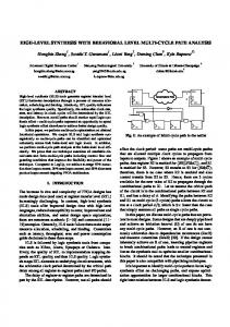
Automata Representation of PSL This chapter will provide the prerequisites needed for understanding the automata construction for PSL and will identify the differences between syntactic and semantic automata as well as the impact of these difference on the way automata are handled in the context of PSL. It will also be shown how this relates to pipelining in PSL formulae. After dealing with these prerequisites, an overview to the automata construction for PSL itself will be provided, as outlined in Fig. 4.1: it will be shown that the language is composed of a set of base cases, denoted PSLmin , and rewriting rules that allow converting PSL’s more complex constructions to PSLmin . Then, automata generation algorithms for PSLmin will be pointed out, and finally an algorithm to perform the necessary conversions of the constructed nondeterministic automata so that they are capable of dealing with both pipelining and the semantics of PSL will be presented. PSL Assertion Assertion in PSLmin Nondeterministic Automaton Deterministic Automaton Implementation Figure 4.1: The way from an assertion to a HDL implementation of a checker simulating the assertion.

24

CHAPTER 4. AUTOMATA REPRESENTATION OF PSL

25

0

qa

1 0

1 qb 0

1 qc

Figure 4.2: A simple deterministic automaton consisting of three states (vertices) qa , qb and qc and six transitions (edges).

4.1

Automata Theory

In order to understand the underlying aspects of PSL, one needs basic knowledge of automata theory, which is a part of the theory of computation. Most books covering the theory of computation devote a large part to automata theory [Sip06, HMU01, Gop06]. Automata consist of states and transitions connecting the states. The current state can be viewed as the memory of a computer and the transitions are the way the computer reacts to different input symbols. Therefore, automata provide a simple and intuitive way to describe sequences which are discrete in time. Directed graphs are usually used to visualize an automata in a so-called state diagram: the automaton’s states are depicted as the vertices and the transitions as the edges; see Fig. 4.2 for an example. In the simplest case (which will be defined as a deterministic automaton in Sec. 4.1.1), every state of an automaton has exactly one outgoing transition for every possible input symbol. The state in the state diagram drawn with a bold outline is called the start state; this is the state in which the automaton starts its computation. If an automaton is in a given state and an input symbol is received, it computes its next state by traversing the current state’s outgoing transition labeled with the received input symbol. As soon as the next symbol is received, the automaton computes its next state again, thus creating a state sequence (or state trajectory) σ = q0 q1 . . . of locations in Q, which is the set of the automaton’s states [RFB05]. Automata are said to accept an input string (which is a concatenation of one or more input symbols) if, after processing all input symbols, the current state of the automaton is a so-called final or accept state 1 , which is drawn as a double circle in the state diagram. In other words, an automaton 1

This definition is obviously only applicable to automata that are restricted to finite input strings. For automata that need to be able to handle infinite input words, socalled B¨ uchi-automata, this definition needs to be changed: such an automaton accepts an infinite input word if it visits accepting states infinitely often [BBF+ 05, Var95]. For the sake of simplicity, no distinction between those two types of automata will be made in the following sections—the correct determination will be implicitly applied.


26

accepts an input string if and only if σ = q0 q1 . . . qn so that qn ∈ F , where F is the set of the automaton’s final states. Given that knowledge, it can be determined that the automaton in Fig. 4.2 accepts the strings 11 (σ = qa qb qc and qc ∈ F ), 011 (σ = qa qa qb qc and qc ∈ F ), 01011 (σ = qa qa qb qa qb qc and qc ∈ F ), and any other string ending with 11. The input string 00, for example, is not accepted since the state trajectory is σ = qa qa qa , so the automaton stops in state qa which is not a final state (qa ∈ / F ). The set of all strings that an automaton A accepts is called L (A) or the language of A [RFB05, Sip06]. Formally, a finite automaton can be described using a 5-tuple A = (Q, Σ, δ, q0 , F ) [HMU01, Sip06]: 1. Q is a finite set of states. 2. Σ is a finite set of input symbols, called the input alphabet. 3. δ ⊆ Q × Σ × Q is the set of transitions or transition relation. Alternatively, δ is often defined as a transition function δ = Q × Σ −→ Q. Those two notations are equivalent; each definition can be used to describe the other (let δr be the transition relation and δf be the transition function): δf (q1 , l) = {q2 | (q1 , l, q2 ) ∈ δr }. With a few exceptions, in which it is favorable to use the transition function, the transition relation will be used throughout this work. 4. q0 ∈ Q is the start state. 5. F ⊆ Q is the set of final states. The transition relation δ describes all edges of the automaton. Informally, an edge e = (q1 , l, q2 ) ∈ δ is the edge the automaton traverses when its current state is q1 and the input symbol is l; therefore, the automaton’s next state will be q2 . Returning to the example in Fig. 4.2, one can describe the automaton as A1 = (Q, Σ, δ, q0 , F ) where: 1. Q = {qa , qb , qc }, 2. Σ = {0, 1}, 3. the transition relation δ is defined by

δ = {qa , 0, qa } , {qa , 1, qb } , {qb , 0, qa } , {qb , 1, qc } ,

{qc , 0, qa } , {qc , 1, qc } , 4. q0 = qa , and

CHAPTER 4. AUTOMATA REPRESENTATION OF PSL 1

qa

27

0 1

qb

qc

Figure 4.3: A nondeterministic automaton consisting of three vertices and three transitions.

5. F = {qc }. The language of A1 is, as mentioned before, the set of all strings the automaton A1 accepts, therefore: L (A1 ) = {l1 , l2 , . . . , ln | ∀li : li ∈ Σ and ln = 1 and ln−1 = 1} .

4.1.1

Deterministic Finite Automata

Deterministic finite automata (DFA) are, as previously stated, the simplest case of automata. They can easily be implemented in hardware and the automaton always has exactly one current state and therefore for a given input string exactly one state sequence σ exists. Formally, an automaton A is called deterministic if and only if 1. every2 state q1 ∈ Q has exactly one outgoing transition (q1 , l, q2 ) ∈ δ (q2 ∈ Q) for each symbol l ∈ Σ and 2. there are no transitions (q1 , , q2 ) ∈ δ for any q1 ∈ Q and q2 ∈ Q. The input symbol matches the empty string—this will be explained in detail in Sec. 4.1.2. Nonetheless, it is worth noting that any automaton that has an -transition is not a deterministic automaton. In the following sections, D will be used to denote deterministic automata.

4.1.2

Nondeterministic Finite Automata

Nondeterministic finite automata (NFA, denoted as N ) are a generalization of deterministic finite automata. In an NFA, several different possible state trajectories may be possible for a single current state and a given input word. The automaton presented in Fig. 4.3 is an example of an NFA: state qa has two outgoing transitions for 1 but none for 0, qb has no transition for 1 but one for , and qc has no outgoing edge at all. Given a deterministic automaton, the state trajectory the automaton traverses when it is fed a given input string is predefined (i. e. exactly one 2

As a simplification, final states are often omitted in this rule.


28

possible state trajectory exists) and can easily be determined. Obviously, this is not as simple with an nondeterministic automaton—for the example in Fig. 4.3, what does the automaton do when it is in state qa and the input is 1? What does it do when the input is 0? How and when does the automaton traverse -edges? The answer to the first two questions is simple: if the automaton is in state qa and the input is 1, its next state is both state qa and qb . If the input is 0, however, its next state is no state at all. Given this, one can conclude that an NFA can be in any combination of its states (including no state at all) simultaneously. When the automaton cannot deterministically decide in which state to traverse, one can think of the automaton “branching”: if its state is qa and the input is 1, the automaton copies itself and one instance goes to state qa while the other one goes to state qb . Another possible view, which is the one used in the formal specification, is that a nondeterministic automaton can be in a set of states at the same time. To answer the third question, it is helpful to return to the definition of . It is the empty string, therefore its length || = 0. This means that such an edge can be traversed without an input symbol—therefore, an -transition (q1 , , q2 ) is traversed as soon as the state q1 is reached. For our example, this means that if the automaton is in state qa and the input is 1, the new state of the automaton comprises not only of the states qa and qb , but also, since qb is activated, of qc . Formally, a nondeterministic automaton N is, just as its deterministic counterpart, a 5-tuple N = (Q, Σ, δ, q0 , F ), but δ is defined slightly differently: 1. Q is a finite set of states, 2. Σ is a alphabet, 3. δ ⊆ Q × Σ × P (Q) is the transition relation3 , 4. q0 ∈ Q is the start state, and 5. F ⊆ Q is the set of final states [HMU01, Sip06]. This modification of δ enables the automaton to comprise of transitions from one state to a set of states. Returning to our example, one can define the automaton in Fig. 4.3 as N1 = (Q, Σ, δ, q0 , F ), where: 1. Q = {qa , qb , qc }, 2. Σ = {0, 1}, 3

P (Q) denotes the powerset of Q.


29

3. the transition relation δ is defined by

δ = {qa , 0, ∅} , {qa , 1, {qa , qb }} , {qb , 0, {qb }} , {qb , 1, ∅} , {qb , , {qc }} ,

{qc , 0, ∅} , {qc , 1, ∅} , 4. q0 = qa , and 5. F = {qc }. Nondeterministic finite automata can be implemented in hardware very efficiently, even without converting them to DFA (how this can be done will be presented in 4.1.4). Nonetheless, in Sec. 4.3 it will be shown that implementing the NFA directly is impossible when constructing automata for PSL.

4.1.3

Regular Languages and Regular Expressions

As mentioned before, the set of strings an automaton A accepts is called the language of A or L (A); all languages that are accepted by either an NFA or a DFA (it will be shown in Sec. 4.6 that NFAs can be used to simulate DFAs and vice versa) are called regular languages. Three basic operations are defined for languages, let L1 and L2 be languages [HMU01, Sip06]: 1. Union: L1 ∪ L1 = {x | x ∈ L1 or x ∈ L2 }, 2. Concatenation4 : L1 ◦ L2 = {xy | x ∈ L1 and y ∈ L2 }, and 3. Kleene Closure5 : L∗ = {x1 x2 x3 . . . xk | k ≥ 0 and each xi ∈ L}. As additional terminology, define that if w = xy, x is a prefix of w, denoted x w, and y is a suffix of w, and w is an extension of x, denoted w x. w0 is defined as the first letter of w. Moreover, if L = L (A), let L0 = {} and Li = L ◦ Li−1 for i ≥ 1 [RFB05]. One can use regular expressions to describe regular languages. Therefore, automata can be used to define a regular expressions and vice versa: for every regular expression, there exists a nondeterministic automaton that accepts the same language and is linear in the regular expression’s size [BFR05]. Regular expressions can be defined inductively; if r1 and r2 are regular expressions, then r is a regular expression if: 1. r = a for some a in Σ, 2. r = , 4 5

The concatenation operation is often just denoted L1 L2 instead of L1 ◦ L2 . The Kleene Closure is also called the Kleene Star or simply star operator.


30

3. r = ∅, 4. (r1 ∪ r1 ), often denoted as (r1 |r2 ), 5. (r1 ◦ r2 ), often denoted as r1 r2 , and 6. (r1∗ ) [Sip06]. Languages can be derived from a regular expression using the following rules: • L (b) = {b}, • L () = {}, • L (∅) = ∅, • L (r1 ∪ r2 ) = L (r1 ) ∪ L (r2 ), • L (r1 ◦ r2 ) = L (r1 ) L (r2 ), and • L (r∗ ) = L (r)∗ [RFB05]. This shows that both the usage of regular expressions and regular languages and the operations on them are analogous; therefore, they are sometimes used interchangeably. Describing languages using regular expressions is intuitive and straightforward. Suppose one wants to describe the language “any string that ends with 11”, which is what the automaton given in Fig. 4.2 accepts: the regular expression for this language (over the alphabet Σ = {0, 1}) is Σ∗ 11, which denotes an arbitrary count (including zero) of any character in Σ followed by 11.

4.1.4

Converting NFA to DFA

Nondeterministic finite automata are a generalization of their deterministic counterparts; it is therefore obvious that they can simulate the behavior of a DFA. On the other hand, which is less obvious, DFAs can also be used to simulate NFAs. Simulated, in this case, means that it is possible to construct a DFA that, despite having a different structure, reacts in precisely the same way to any arbitrary input string as the NFA would (i. e. they accept the same language); both automata are said to be equivalent [Sip06]. As previously mentioned, an NFA can be in any subset of its states at a single point in time: if it has k states, there are 2k possible subsets of these states [Sip06]. Converting it to a DFA involves denoting every subset of those states with a single state, i. e. constructing a DFA with 2k states6 . 6

In practice, though, in many cases a lot of those states are unreachable, which means that there is no input word so that the automaton could reach one of those states. Therefore, they can be easily dropped using an optimization algorithm (see Sec. 5.4).


31

This means that the created DFA is exponential in the size of the NFA, which is consistent with the findings about LTL formulae in [KV99], and, since LTL is a subset of PSL, also holds for PSL [RFB05]. Formally, the construction for a DFA D = (QD , ΣD , δD , q0,D , FD ) simulating an NFA N = (QN , ΣN , δN , q0,N , FN ) is, as shown by Sipser [Sip06]: 1. QD = P (QN ): the states of D are all possible combinations of the states in N . 2. ΣD = ΣN : the input alphabet is (obviously, since both automata should behave in the exact same way) identical. 3. δD : For the sake of completeness, the definition of the -reachability (or -closure as defined by Hopcroft et al. [HMU01]) E is necessary:

E (R) = q | q can be reached from R by traveling along

0 or more arrows

If R ∈ QD (i. e., R ⊆ QN ) and a ∈ ΣD , then define7 δD (R, a) = {q ∈ QN | q ∈ E (δN (r, a)) for every r ∈ R} . If, for the automata construction algorithms for PSLmin , as presented in Sec. 4.4, would use -transitions, the automata conversion algorithms would need to be extended to use the -closure. Omitting -transitions during the construction eases both the process of converting and minimizing the automata. Therefore, no algorithms presented for PSL automata construction generate any -transitions and, consequently, the -closure can be ignored. This simplifies the equation given above to δD (R, a) = {q ∈ QN | q ∈ δN (r, a) for every r ∈ R} . 4. q0,D = E (q0,N ): the start state of D is the set of states containing the start state of N and all states that are within this state’s -reachability. Again, since the algorithms presented for PSLmin automata construction do not generate -transitions, the -closure can be omitted, simplifying the equation to q0,D = q0,N . 5. FD = {R ∈ QD | ∃r ∈ R so that r ∈ FN }: every state in D that contains at least one final state of N is a final state for D. 7 Note that in this equation, the transition function δ = Q × Σ −→ Q, instead of the transition relation δ = Q × Σ × Q, is used for the sake of simplicity.


4.1.5

32

Additional Operations on Automata

This section covers two additional functions which can be used on automata: outgoing (S) and incoming (S). They will be used in both automata construction for PSL and automata conversion. Let q be a state and S be a set of states. outgoing (q) = {(q1 , l, q2 ) ∈ δ | q1 = q} incoming (q) = {(q1 , l, q2 ) ∈ δ | q2 = q} outgoing (S) = {(q1 , l, q2 ) ∈ δ | q1 ∈ S} incoming (S) = {(q1 , l, q2 ) ∈ δ | q2 ∈ S} Those functions determine all outgoing or incoming edges to a given state or set of states.

4.1.6

Summary

This section outlined the basics of automata theory. Deterministic automata are the simplest form of an automaton and their state trajectory is welldefined for any given input. Nondeterministic finite automata are a generalization that allow transitions for the empty string , transitions to different states for the same input character l ∈ Σ, and states without transitions for one or more given input characters l ∈ Σ. This leads to the fact that an NFA can be in any arbitrary number of its states at once, which is (in software) often implemented as branching. Furthermore, with regular languages and regular expressions a convenient form of representing automata that recognize a given set of strings was presented. Finally, the relationship between deterministic and nondeterministic finite automata was shown, including the fact that both can be simulated by their counterpart. Moreover, the functions outgoing (S) and incoming (S) were defined to easily determine the outgoing and incoming edges of a given state or set of states.

4.2

Language and Semantics of Regular Expressions

As shown in Sec. 4.1.3, regular expressions can be used to define regular languages. This approach includes one basic assumption: every time an input symbol is received, only one input symbol is received. In other words, it is impossible for two different input symbols to be received at the same time.


33

For conventional finite automata, as widely used in pattern recognition [Nav01, CPZ99, BK92, AA04], this assumption is hardly a restriction: pattern matching usually works on an input string which is a sequence of characters. Formally, the language of the intersection of any two characters a and b (a 6= b) is given by L (a ∩ b) = L (a) ∩ L (b) = ∅, which means that all characters in a given alphabet Σ are disjoint and that an input character can either be one or another character, but not two different characters at the same time [RFB05]. In PSL, though, regular expressions need to be viewed in a semantic way. In order to understand this view, some identifiers as defined by Ruah [RFB05]8 are needed. Let V be a set of state variables and define ΣV as the set of all states that the state variables in V form (these definitions were used similarly by Kesten et al. [KPR98] for fair Kripke structures). ˆ V = ΣV ∪ {>, ⊥} and BV to be the set of boolean expresAlso, define9 Σ sions over V (this was defined by Bohn et al. as B(V ) [BDG+ 98]). Boolean satisfaction is defined as l b ⇐⇒ l ∈ b, > b, and ⊥ 3 b for any letter l ∈ ΣV and any boolean expression b ∈ BV . Moreover, analogously to L for the language described by a regular expression, define S to be the semantics of a regular expression over boolean expressions. The semantics of the intersection of two letters a and b is given by n

ˆ ∗V | |w| = 1 and w S (a ∩ b) = w ∈ Σ

a and w

o

b 6= ∅,

which, in essence, means that a given letter l ∈ ΣV can satisfy both a and b at the same time [RFB05, BFH05], or, informally, be the combination of a and b. As an example, let Nr = (BV , Q, δ, q0 , F ) be a traditional (“syntactic”) NFA that accepts the language L (r) if r is a given regular expression. If, for instance, r = ab∗ c, then the word w1 = abc ∈ L (r) is accepted by Nr . The word w2 = (a ∧ b)bc, on the other hand, is not accepted by Nr (and in the traditional definition of automata theory not even possible), since w2 ∈ / L (r) [RFB05]. A “semantic” NFA should accept both w1 and w2 , though—remember that, in this case, a, b and c are three different Boolean variables that may be true at the same time. This distinction leads to some differences in interpreting automata for PSL as opposed to widely used traditional approaches that only consider 8

This section aims to provide a short overview of the semantics of regular languages, not a complete formal definition. The exact definitions can be found in the documents referred to. 9 > and ⊥ are defined by Eisner et al. [EFHM06]. Basically, both > and ⊥ are special letters that satisfy all Boolean expressions or no Boolean expression at all, respectively. They are needed for reasoning over truncated paths.


34

a

qa

b

qb

Figure 4.4: An automaton that recognizes L (a∗ b). It is deterministic in its syntactic sense but nondeterministic in its semantic sense [RFB05].

languages (e. g. [Sip06, HMU01, Gop06]). The foremost discrepancy lies in the interpretation of automata: an automaton that is deterministic judged by its language may very well be nondeterministic judged by its semantics. For instance, the automaton in Fig. 4.4 (taken from Ruah et al. [RFB05]) over the alphabet Σ = {a, b} is deterministic in its syntactic sense (N = Nr ), but not in its semantic sense (N = Ns ). This becomes obvious when considering that the alphabet of Ns is defined as ΣV which is defined as the set of states formed by the variables in V = {a, b}, therefore ΣV = {∅, {a} , {b} , {a, b}}. This means, that instead of a and b being elements of Σ, they are elements of V and can therefore hold at the same time. Summing up, a challenge encountered while constructing automata for PSL is that the traditional automata theory does not cover the semantics of regular expressions over boolean expressions, but only the syntax of the input strings. Therefore, the construction, and in particular the conversion of an NFA to a DFA, needs to be slightly modified in order to produce behavior consistent with PSL’s semantics. These modifications will be presented in Sec. 4.6.

4.3

Pipelining in PSL Formulae

The difference between the semantics of a regular expression and its language described in the last section leads to another aspect of PSL that is not covered in conventional automata theory: pipelining, which means that the very pattern that is just recognized can start again before the recognition of the first word is finished (and the word either accepted or denied). Again, for commonplace pattern recognition applications, this is not a restriction, since every two characters of an alphabet are disjoint and therefore cannot occur simultaneously. However, Looking at a simple PSL property, it becomes obvious that this needs to be considered in the context of PSL. For example, consider the property always ({b1 } |=> {b2 [∗2]; b3 }) and the trace shown in Fig. 4.5. The postcondition is triggered three times and holds three times, namely in cycles 4, 6, and 7. It is obvious that the checker needs to be able to deal with the pipelining introduced by this behavior.


35

1 2 3 4 5 6 7 8

b1 b2 b3

| {z } (1)

| {z } (2)

| {z } (3)

Figure 4.5: The property always ({b1 } |=> {b2 [∗2];b3 }) is triggered three times; the checker needs to support pipelining. 1 2 3 4 5 6 7 8

b1 b2 b3 Figure 4.6: The property always ({b1 } |=> {b2 [∗];b3 }) is triggered four times. It holds four times, too—all four times being in cycle 7.

This behavior has even more impact when considering the property always ({b1 } |=> {b2 [∗]; b3 }). See trace 4.6: the postcondition is triggered in cycles 2, 4, 5, and 7, and it holds four times, all four times being in cycle 7. This means that multiple start conditions may very well finish in the same cycle, therefore creating only one hold or only one fail signal, or, even, both the hold and the fail at the same time.

4.3.1

Pipelining and Nondeterministic Automata

Return to the basic difference between nondeterministic and deterministic automata: an NFA can be in a set of states at once, a DFA only in one state at a time. As previously maintained, NFA can be implemented in hardware very efficiently: a state can be modelled as a flipflop and transitions are simply enable signals for those flipflops. For the (semantically nondeterministic!) automaton presented in Fig. 4.7, one would need three flipflops and three “and” gates to model its behavior10 ; the schematic is shown as seen in Fig. 4.8. This implementation follows the idea that an NFA can be in a set 10 It is interesting to note that the implementation using atomic checkers, as presented by Das et al. [DMDC06] and elaborated in Sec. 3.1, would produce the same result for {b1 ;b2 ;b3 }: compare the schematic presented in Fig. 4.8 to one generated using atomic checkers as for example given in Fig. 3.2. In fact, the automata approach is a generalization of the approach based on atomic checkers.

36


qa

b1

qb

b2

b3

qc

qd

Figure 4.7: A semantically nondeterministic automaton for {b1 ;b2 ;b3 }.

’1’

DFF qa

&

DFF qb

&

DFF qc

&

DFF qd

accept

b1 b2 b3

Figure 4.8: Efficient hardware implementation of the NFA given in Fig. 4.7.

of states; in the given implementation, every state is a flipflop, therefore the automaton can be in a set of states too. This straightforward way of implementing an NFA detects even pipelined occurrences of the given sequence, but it still bears a basic problem: since the automaton can be in a set of states at a single time (which corresponds to several flipflops outputting ’1’ at the same time), one cannot know which active state was caused by which activation of the automaton. Considering that multiple start conditions can occur before a sequence finishes, this leads to the fact that one cannot determine if and when the automaton should reject the given input (i. e. assert the “fail”-signal): a sequence is rejected if the last branch of the NFA dies, which it does as soon as there is no more active state caused by the sequence’s start condition. This is impossible to detect, though, since one cannot determine which active state was caused by which start condition. The same problem occurs with sequence acceptance: once the sequence was accepted for the first time, it can be desirable to terminate the recognition. The sequence {b1 ; b2 [+]}, for example, can be accepted infinitely often for a single start condition, but signalling only the first match may be enough and signalling all other matches may even be unwanted. Terminating a run of the NFA would mean terminating all other branches that were triggered by this run’s start condition. Therefore, it would require removing all active states that were caused by this start condition. However, this is impossible, since once again one cannot know which start condition caused a given state in the automaton to be activated. It becomes obvious that the problems encountered are directly caused by the branching of the NFA. Since branching is the very thing that makes an NFA nondeterministic, converting it to a DFA suggests itself: a DFA is in only one state, or, in other words, it does not branch. If, for a given input, there is no successor state for an active state, this branch “dies”; therefore


37

the input word was rejected and the “fail”-output can be asserted11 . On the other hand, one can also easily terminate the automaton after it accepted a string for the first time by simply removing the outgoing transitions from all final (accepting) states. As a result, it is obvious that, in PSL’s context, automata cannot be implemented as NFAs but need to be converted to DFAs.

4.4

PSLmin : Base Cases and Rewriting Rules

Before the first standardization of PSL by Accellera [Acc03], the language was developed by IBM under the name Sugar [EF02]. This name was chosen for the fact that the language offers few possibilities that its base language (which, as mentioned by Eisner and Fisman [EF06], was CTL before the committee moved to LTL because of Vardi’s findings, e. g. [Var01]) did not yet provide. Sugar just added a lot of so-called “syntactic sugaring” to facilitate and ease the process of writing those formulae and, at the same time, make them more easily understood. Therefore, most of PSL’s statements can be rewritten to a relatively small amount of base cases, which will be denoted PSLmin . On the one hand, rewriting the formulae makes them less succinct, but, on the other hand, allows for easier implementation: a tool dealing with PSL can rewrite those complex properties to the base cases and only provide implemention algorithms for these. The following section provides an overview of the rewriting rules as presented in the LRM [Acc04a] and the work of Boulé and Zilic [BZ06].

4.4.1

Boolean Layer

The Boolean layer comprises all expressions that are Boolean—this includes signal names as well as HDL expressions (for example, any HDL terms) and PSL expressions (especially all built-in function calls like, for example, prev(b) and rose(b) and the logical implication and “iff” operators) [EF06]. Let b be a Boolean expression and c a positive integer. 4.4.1.1

Base Cases (Part of PSLmin )

All HDL expressions can be implemented directly and, therefore, are base cases. prev(b, c) is implemented as c flipflops through which b is fed. 11

To achieve this, a new state qsink is added during the conversion from NFA to DFA.

CHAPTER 4. AUTOMATA REPRESENTATION OF PSL 4.4.1.2

38

Rewriting rules b1 −> b2 b1 b2 prev(b) rose(b) fell (b) stable(b)

≡ ≡ ≡ ≡ ≡ ≡

(not b1 ) or b2 (b1 −> b2 ) and (b2 −> b1 ) prev(b, 1) b and not prev(b) (not b) and prev(b) prev(b) b

Notes: • The built-in functions countones, onehot, and onehot0 can be implemented directly in HDL code. • The built-in function isunknown checks a Boolean expression or a vector for occurrences of “unknown” values (i. e., any values other than ’0’ and ’1’ ) [Acc04a]. Therefore, implementing it in hardware is not sensible: the tri-state value ’Z’ is the only value other than ’0’ and ’1’ that can occur in hardware. However, checking for ’Z’ is difficult in hardware and using tri-state signals on-chip is mostly considered bad design pratice. Moreover, tri-state signals are usually implemented using three signals: input, output, and output-enable. These three signals can easily be checked with assertions in both simulation and hardware.

4.4.2

SEREs and Sequences

The temporal layer contains Sequential Extended Regular Expressions which allow describing the relation between Boolean layer expressions over time. Let r be a SERE, b a Boolean layer expression, and c, l and h integers where l and h describe the lower and upper bound of a range (and therefore h ≥ l), respectively. 4.4.2.1

Base Cases (Part of PSLmin ) {b} r[∗] {r1 ;r2 } {r1 :r2 } r [∗0] r[∗l to h] r1 | r2 r1 && r2


39

Notes: • The base case r[∗0] is equivalent to [∗0] and was denoted a “degenerate SERE” by Eisner et al. [EFH03a], but that remark is no longer available in the LRM [Acc04a]. The formal semantics of PSL describe [∗0] as v |≡ [∗0] ⇐⇒ v = , which, informally, means that the empty string and only the empty string satisfies [∗0] . Therefore, a special implementation of [∗0] is not needed as [∗0] corresponds to an -Transition. • Both the LRM [Acc04a] and Boulé and Zilic [BZ06] propose rewriting r[∗l to h] as r[∗l] | r[∗l+1] | . . . | r[∗h]. This approach is not used, since it leads to higher implementation efforts; “ranged SEREs” are handled as a base case because they can be implemented very efficiently, as will be shown in Sec. 4.5.3.6. 4.4.2.2

Rewriting Rules r[+] r[∗c] b[−>] b[−>c] b[−>l to h] b[=c] b[=l to h] r1 & r2 r1 within r2

≡ ≡ ≡ ≡ ≡ ≡ ≡ ≡ ≡

r;r[∗] r;r;. . .;r

(c times)

{not b[∗]; b} {b[−>]}[∗c] {b[−>]}[∗l to h] {b[−>c]}; not b[∗] {b[−>l to h]}; not b[∗] {{r1 ; [∗]} && {r2 }} | {{r1 } && {r2 ; [∗]}} {[∗]; r1 ; [∗]} && {r2 }

Note: • Rewriting r1 & r2 as {r1 ; [∗]} && {r2 ; [∗]} might seem favorable, but is not accurate: after both r1 and r2 have finished, this rewriting rule would give an infinite amount of matches (if it is not terminated after the first one, obviously; see Sec. 4.5.4.4 for details), which is incorrect.

4.4.3

Properties

Properties can be used to describe behavior. Let p be a property, b be a Boolean expression, and r be a SERE.


40

Base Cases (Part of PSLmin ) b r p abort b p1 && p2 r |−> p r |=> p p until b r! eventually! r

Notes: • p1 && p2 can be implemented in the same way as r1 && r2 since both properties and sequences are represented using automata. • The LRM [Acc04a] and Boulé and Zilic [BZ06] suggest implementing r |=> p as a simple suffix implication {r; true} |−> p which is obviously possible but not always desirable since r |=> p itself may be easier to implement than r |−> p. • The property p until b can, informally, be rewritten to {p[∗]; b}. Note that this rule is formally incorrect since properties cannot be used as SEREs, therefore neither the Kleene Closure nor the SERE concatenation can be applied to them. Nonetheless, this rewriting rule can be applied since the approach presented converts properties to automata, just as it does with SEREs; on automata level both can be handled in the same way. • The elements below the line are strong sequences and strong properties, i. e. r! and eventually! r, and can be implemented, as shown by Boulé and Zilic [BZ06], by adding an additional “end-of-simulation” signal to the checker.


41

Rewriting Rules b −> p b or p {r}(p) b1 until b2 b1 before b2 b1 before b2 next p next[c] p next a[l to h] p next e[l to h] p next event(b)(p) next event(b)[c](p)

next event a(b)[l to h](p) next event e(b1 )[l to h](b2 ) always p never r p until! b b1 until! b2 b1 before! b2 b1 before! b2 next! p next![c] p next a![l to h] p next e![l to h] p next event!(b)(p) next event!(b)[c](p) next event a!(b)[l to h](p) next event e!(b1 )[l to h](b2 ) eventually! r

≡ ≡ ≡ ≡ ≡ ≡ ≡ ≡ ≡ ≡ ≡ ≡ ≡ ≡ ≡ ≡ ≡ ≡ ≡ ≡ ≡ ≡ ≡ ≡ ≡ ≡ ≡ ≡ ≡

{b} |−> p (not b) −> p r |−> p {b1 [∗]; b1 and b2 } {(not b1 and not b2 )[∗]; (b1 and not b2 )} {(not b1 and not b2 )[∗]; b1 } next[1] p next event(true)[c+1](p) next event a(true)[l+1 to h+1](p) next event e(true)[l+1 to h+1](p) next event(b)[1](p) next event a(b)[c to c](p) {b[−>l to h]} |−> (p) {b1 [−>l to h] : b2 } {[+]} |−> p {[+] : r} |−> false (p until b) : ({b[−>]}!) {b1 [∗]; b1 and b2 }! {(not b1 and not b2 )[∗]; (b1 and not b2 )}! {(not b1 and not b2 }[∗]; b1 }! next![1] p next event!(true)[c+1](p) next event a!(true)[l+1 to h+1](p) next event e!(true)[l+1 to h+1](p) next event!(b)[1](p) next event a!(b)[c to c](p) next event a(b)[l to h](p) && {b[−>h]}! {b1 [−>l to h] : b2 }! {[+] : r}!

Notes: • The property {r}(p) is semantically equivalent to r |−> p [Acc04a]. • Boulé and Zilic define the rewriting rule for b1 until b2 using SERE fusion as {b1 [+] : b2 } [BZ06], but without optimizations on the generated automaton the fusion operator is more complex in its implementation (with optimizations both solutions are equivalent). • All items below the line are liveness properties that need an end-ofsimulation signal as mentioned before.


4.5

42

Construction of NFAs for PSLmin

As shown in Sec. 4.4, complex PSL constructs can be rewritten to simple base cases, denoted PSLmin , that provide the same functionality. Therefore, it is sufficient to find appropriate implementations for PSLmin —all other possibilities provided by PSL can be easily mapped to them. In the following section algorithms for efficiently constructing NFAs for PSLmin will be shown. Note that the following automata are nondeterministic and only implement base cases; therefore, neither distinction between syntactic and semantic automata or pipelining need to be considered at this stage: this will be taken care of when converting the constructed NFAs to DFAs. Nonetheless, keep in mind that, as outlined in 4.2, the transitions are labeled with elements of BV and not with elements of ΣV , which means that different labels can be satisfied at the same time. Also, note that all automata presented in the following section only accept an input word; they do not specifically reject it if it is not accepted. This is of course needed, but this behavior will be added by extending the states of the automaton to an additional sink state while converting the constructed NFA to a DFA (see Sec. 4.6). All of the following algorithms construct automata that do not comprise -transitions. Using them would, on the one hand, simplify many constructions, most notably automata concatenation and disjunction, but on the other hand -transitions increase the amount of generated states and therefore increase calculation time as well as the reliance on the optimization done by the synthesis tool.

4.5.1

Preliminaries

This section presents the construction of automata for each base case of PSLmin , both informally and formally. First, however, the identifiers and the clock context used need to be defined. 4.5.1.1

Identifiers

Boolean expressions will be denoted with b, SEREs with r, properties with p, positive integers with c, l, and h, input strings with w, nondeterministic finite automata with N , and deterministic finite automata with D. In graphical representations of automata a bold outline will be used to denote the automaton’s start state. Double-circled states will again be used to denote final states. Transitions will be labeled with elements of BV .


DFF

b

DFF

DFF

43

prev(b, c)

clk

| c

{z times

}

Figure 4.9: Implementation of prev(b,c).

4.5.1.2

Clocked and Unclocked Semantics of PSL Properties

PSL foundation language properties need not define a clock expression under which they need to be evaluated. This is useful for e. g. formal verification, but hardly makes sense for functional verification in a synchronous sequential environment12 . Therefore, all PSL formulae, automata, and examples presented in this chapter refer to the clocked semantics. For the sake of simplicity, this is not mentioned afterwards.

4.5.2

Boolean Layer

As stated in Sec. 4.4.1.1, all HDL expressions can be implemented directly in hardware, therefore no automata construction is needed for these. prev(b, c) is implemented as shown in Fig. 4.9.

4.5.3

SEREs

This section outlines the automata construction for SEREs and the operations defined on them. 4.5.3.1

Boolean Expressions

An automaton NB accepting a Boolean expression b can be constructed as shown in Fig. 4.10. Since qa is not an accepting state and qb has no outgoing edges, the automaton NB accepts only input strings with a length of exactly one character, thus |w| = 1. Therefore, the automaton accepts an input string w if and only if |w| = 1 and w0 |= b which complies with PSL’s semantics [BBF+ 05, Acc04a]. 4.5.3.2

Kleene Closure

Given an automaton Nr = (Qr , BV , δr , q0,r , Fr ) which accepts the SERE r, the automaton NKleene = (QKleene , BV , δKleene , q0,Kleene , FKleene ) which accepts the Kleene closure r∗ can be constructed as follows [BBF+ 05]: 12 In fact, for functional verification, if there is no clock expression given, the tool applies its own internal granularity of time [Acc04a].


qa

b

44

qb

Figure 4.10: NFA NB that accepts {b}. b

b qa

q0

b qb

b (a)

b

q0

b

qa

(b)

Figure 4.11: (a) Unoptimized and (b) optimized NFA NKleene for {b[∗]}.

1. Create a new state q0 . 2. Let QKleene = Qr ∪ {q0 }, 0 3. and δKleene = δr ∪ {(q0 , l, q2 ) | (q1 , l, q2 ) ∈ outgoing (q0,r )} to create edges from the new start state to all possible successor states of the old start state. 0 4. Let δKleene = {(q1 , l, q0 ) | (q1 , l, q2 ) ∈ δKleene and q2 ∈ Fr } to generate edges from the ancestor states of all final states to the new start state, thus closing the loop.

5. Finally, let q0,Kleene = q0 and 6. FKleene = Fr ∪ {q0 }. This calculation leads, if for example r = {b}, to an automaton as shown in Fig. 4.11a. This automaton can obviously be optimized: since state qa is unreachable, the dashed parts of the automaton can be removed. This optimization leads to the automaton presented in 4.11b. As another example, the optimized automaton for r = {b1 ; b2 } is shown in Fig. 4.12.


q0

b1

qa

b2

45

qb

b2 Figure 4.12: Optimized NFA NKleene for {{b1 ;b2 }[∗]}

4.5.3.3

SERE Concatenation

An automata for {r1 , r2 } accepts an input word w if and only if two words u and v exist so that u w and w = uv and u |≡ r1 and v |≡ r2 . If two SEREs, r1 and r2 , and the respective automata that accept them, N1 = (Q1 , BV,1 , δ1 , q0,1 , F1 ) and N2 = (Q2 , BV,2 , δ2 , q0,2 , F2 ), are given, the resulting automaton Nconcat = (Qconcat , BV,concat , δconcat , q0,concat , Fconcat ) is, as shown by Ben-David et al. [BBF+ 05], defined by: 1. Qconcat = Q1 ∪ Q2 , 2. BV,concat = BV,1 ∪ BV,2 , 3. δconcat = δ1 ∪ δ2 ∪ {(q1 , l, q3 ) | q1 ∈ F1 and (q2 , l, q3 ) ∈ outgoing (q0,2 )}, 4. q0,concat = q0,1 , and (

5. Fconcat =

F2 F1 ∪ F2

if q0,2 ∈ / F2 , otherwise.

Informally, δconcat consists of all transitions in either automaton as well as additional edges from N1 ’s final states to N2 ’s start state’s possible successors, with their respective labels (see item 3). If the start state of N2 is not a final state, Nconcat accepts some input if and only if it reaches a final state of N2 . If, on the other hand, q0,2 is a final state of N2 this means that |≡ r2 and therefore the word w = u = u is accepted if u |≡ r1 . Thus, in this case, the final states of Nconcat need to be the union of F1 and F2 (see item 5). The proof for the construction as described above was given by BenDavid et al. [BBF+ 05]. An example for an automaton that is constructed for the SERE {b1 ; b2 ; b3 } is given in Fig. 4.13a. It is obvious that this algorithm itself is not optimal, since the dashed states qe , qf , and qg are unreachable. They correspond to the start states of the sub-automata and can simply be removed from the automaton using an algorithm that searches for unreachable states and disposes them. The version of this NFA optimized in this way is shown in Fig. 4.13b.

46


qa

b1 b1

qb

b2

qe b2

qc

b1

qf b1

qd

qg (a)

qa

b1

qb

b2

qc

b3

qd

(b)

Figure 4.13: The (a) unoptimized and (b) optimized NFAs Nconcat for {r1 ;r2 ;r3 }.

4.5.3.4

SERE Fusion

SERE Fusion of two SEREs r1 and r2 (their respective NFAs being N1 and N2 ) is similar to SERE concatenation except that the input triggering transitions leading to the final states of N1 must occur at the same time as the input triggering transitions starting in N2 ’s start state. Conventional automata theory does not cover automata fusion since this operation relies on the semantics of the regular expressions; by only looking at their languages, for an input character to trigger two different transitions, the regular expressions13 of those two transitions must be equivalent. Remember the intersection for two characters a and b in their syntactic sense given in Sec. 4.2 and extend it to the only case in which it is not empty: L (a ∩ b) = ∅ ⇐⇒ a 6= b L (a ∩ b) 6= ∅ ⇐⇒ a = b. This shows that only viewing the languages of the regular expressions, there is no sense in creating an edge that accepts the conjunction of two characters: it would either never be triggered (given that a 6= b) or its label would be redundant (given that a = b). Since, for PSL, the semantics of the regular expressions need to be considered, regular expression conjunction makes sense. Again, remember the intersection of characters in the semantic sense of a regular ex13

Transitions, in this context, only accept single characters, but a single character can also be seen as a regular expression (with its length being 1).

CHAPTER 4. AUTOMATA REPRESENTATION OF PSL pression [RFB05]:

n

ˆ ∗ | |w| = 1 and w S (a ∩ b) = w ∈ Σ V

47

o

a and w

b 6= ∅.

It is obvious that, in PSL’s semantic sense, an input word w of length 1 (i. e., an input letter) can satisfy both a and b even if a 6= b. SERE fusion is often referred to as overlapping concatenation [BBL98, BFR05], where two words w1 and w2 are concatenated with an overlap by using the conjunction of the last letter of w1 and the first letter of w2 [BBL98]; Ben-David et al. use the same definition for Regular LTL (RLTL) [BFR05]. Thus, the automaton Nfusion = (Qfusion , BV,fusion , δfusion , q0,fusion , Ffusion ) accepting the fusion of two SEREs r1 and r2 (their corresponding NFAs being N1 = (Q1 , BV,1 , δ1 , q0,1 , F1 ) and N2 = (Q2 , BV,2 , δ2 , q0,2 , F2 ), respectively) can be constructed as follows (similar algorithms are given by Gheorghita and Grigore [GG05] as well as Boulé and Zilic [BZ07]): 1. Let Qfusion = Q1 ∪ Q2 and 2. BV,fusion = BV,1 ∪ BV,2 . 3. Define δ as

δfusion = δ1 ∪ δ2 ∪ (q1 , l1 ∧ l2 , q2 ) | (q1 , l1 , f ) ∈ δ1

and f ∈ F1 and (q0,2 , l2 , q2 ) ∈ δ2 . 4. Finally, let q0,fusion = q0,1 , and 5. Ffusion = F2 . Note that unlike Fconcat in the construction of an automaton for SERE concatenation, Ffusion does not use a case differentiation for q0,2 ∈ F2 or q0,2 ∈ / F2 —this is because of the semantics as given in the LRM [Acc04a]: {{b1 ; b2 } : {b3 [∗]}} is equivalent to {{b1 ; b2 } : {b3 [+]}} or {{b1 ; b2 and b3 } : {b3 [∗]}}, therefore the state q0,2 cannot be a final state if the SERE is fusioned with another SERE. This problem is based on the way degenerate SEREs are handled in PSL (see Sec. 4.5.3.5). An example for the automata accepting the {{b1 ; b2 } : {b3 ; b4 }} is given in Fig. 4.14. The dashed nodes and edges can be removed after automata construction (note that, even if the automaton is not optimized, q2 is not a final state of Nfusion !). 4.5.3.5

Degenerate SEREs

As shown in Sec. 4.4.2, the SERE r[∗0] can be seen as a degenerate SERE. Remember that the formal semantics for [∗0] (which is obviously equivalent to r[∗0]) are defined in the LRM [Acc04a] as: v |≡ [∗0] ⇐⇒ v =

48


b1

q0

b2

q1

q2

b2 b3

b3

q3

b4

q4

q5

Figure 4.14: NFA Nfusion for {{b1 ;b2 } : {b3 ;b4 }}.

qa Figure 4.15: NFA Nempty for {[∗0]} .

qa

b

qb

b

qc

b

qd

Figure 4.16: NFA Nranged for {r[∗1 to 3]}.

This means that the only string [∗0] accepts is the empty string . Therefore, the simplest automaton accepting this SERE is the one shown in Fig. 4.15. It is obvious that implementing this automaton is not sensible—it needs to be omitted semantically, i. e. the compiler needs to make sure that no such empty SERE can exist. 4.5.3.6

Ranged SEREs

The construction of automata Nranged for ranged SEREs is based on the algorithm for SERE concatenation: a SERE {r[∗l to h]} is implemented as {r[∗l]; r[∗0 to h−l]}. r[∗l] can be implemented using normal SERE concatenation, and r[∗0 to h−l] is implemented as a SERE concatenation r[∗h−l] where not only the final states of the last sub-automaton are the final state of Nranged but all final states of all sub-automata are set as accepting. An example for {r[∗1 to 3]} is shown in Fig. 4.16.


49

SERE Disjunction

If two sub-automata N1 = (Q1 , BV,1 , δ1 , q0,1 , F1 ) with its language14 being L1 and N2 = (Q2 , BV,2 , δ2 , q0,2 , F2 ) with its language being L2 are given, the automaton Ndisj = (Qdisj , BV,disj , δdisj , q0,disj , Fdisj ) which accepts the disjunction of the languages (Ldisj = L1 ∪ L2 ) of both sub-automata can be constructed as follows: 1. Create a new state q0 . 2. Let Qdisj = Q1 ∪ Q2 ∪ {q0 } and 3. BV,disj = BV,1 ∪ BV,2 . 4. Calculate δdisj as follows: δdisj = δ1 ∪ δ2 ∪ {(q0 , l, q2 ) | (q1 , l, q2 ) ∈ outgoing (q0,1 )} ∪ {(q0 , l, q2 ) | (q1 , l, q2 ) ∈ outgoing (q0,2 )} 5. Finally, let q0,disj = q0 and 6. Fdisj = F1 ∪ F2 . As an example, the unoptimized and optimized NFAs for the disjunction of {{b1 ; b2 } | {b3 ; b4 ; b5 }} are shown in figures 4.17a and 4.17b. Another example for {{b1 ; b2 } | {b3 ; b4 }} can be found in Fig. 4.18. 4.5.3.8

Length-Matching SERE Conjunction

Constructing an automaton which accepts strings that are accepted by two different sub-automata is more complex than creating one that is accepted by one of those two sub-automata. It is not sensible to construct an NFA Nconj from the two sub-automata N1 = (Q1 , BV,1 , δ1 , q0,1 , F1 ) and N2 = (Q2 , BV,2 , δ2 , q0,2 , F2 ): the automaton needs to accept the input if both subautomata accept it, i. e. if both subautomata are in an accepting state at the same time. Marking all states as final in which both automata are in a final state involves constructing the Cartesian product of the states of both automata, which is done anyway during the conversion of the NFA to a DFA. It is obviously sensible to combine both steps; therefore, this algorithm will directly generate a DFA Dconj = (QD , BV,D , δD , q0,D , FD ): 1. Create a new state q0 . 14

Actually, for the construction of automata for PSL, one would need to consider the semantics of the automaton, not its language. Nonetheless, as mentioned in the introduction of this section, the problems arising due to the difference between language and semantics are addressed when converting the NFAs to DFAs.

50


qa

b1

qb

b2

qc

b1

q0 b3

qd

b3

qe

b4

qf

b5

qg

(a)

b1 q0

qb

b2

qc

qe

b4

qf

b3 b5

qg

(b)

Figure 4.17:

(a) Unoptimized and (b) optimized automata Ndisj for

{{b1 ;b2 } | {b3 ;b4 ;b5 }}.

2. Let Qconj = Q1 ∪ Q2 ∪ {q0 } and 3. BV,conj = BV,1 ∪ BV,2 . 4. Calculate δconj as follows: δconj = δ1 ∪ δ2 ∪ {(q0 , l, q2 ) | (q1 , l, q2 ) ∈ outgoing (q0,1 )} ∪ {(q0 , l, q2 ) | (q1 , l, q2 ) ∈ outgoing (q0,2 )} 5. Let q0,conj = q0 . 6. Convert the automaton Nconj to an intermediate deterministic automa 0 0 0 , q0 , F 0 ton Dconj = Q0D , BV,D , δD (how this is done will be outlined 0,D D in Sec. 4.6). 7. Let FD = {f | f ∈ FD0 and f ∩ F1 6= ∅ and f ∩ F2 6= ∅}. Informally, 0 this denotes the set of states of Dconj which contain final states15 of 15 Remember that when converting an NFA to a DFA each state of the DFA is a set of states of the NFA.

51

CHAPTER 4. AUTOMATA REPRESENTATION OF PSL both sub-automata16 .

8. Let S = {q | q ∈ Q0D and (q ∩ Q1 = ∅ or q ∩ Q2 = ∅)}. This is the set 0 of states in Dconj which do not contain states of both automata. In such a state one automaton would be in its sink state. 00 : 9. Calculate δD

00 0 0 = δD \ (q1 , l, s) | (q1 , l, s) ∈ δD and s ∈ S δD

(q1 , l, qsink ) | (q1 , l, s) ∈

0 δD

and s ∈ S

∪

This changes all edges originally leading to states in S to lead to the sink state. 10. Let Q00D = Q0D \ S. 11. Let D = {q | q ∈ Q00D and ∀ (q, l, q2 ) ∈ δD : q2 = qsink }. This is the set of states for which all outgoing edges lead to qsink . 12. Calculate δD :

00 00 δD = δD \ (q1 , l, d) | (q1 , l, d) ∈ δD and d ∈ D

(q1 , l, qsink ) | (q1 , l, d) ∈

00 δD

and d ∈ D

∪

This changes all edges originally leading to states in D to lead to the sink state. 13. Let QD = Q00D \ D. 0 0 . 14. Let BV,D = BV,D and q0,D = q0,D

15. Let Dconj = (QD , BV,D , δD , q0,D , FD ). This is the automaton that accepts the conjunction of both regular expressions. As an example, consider the two regular expressions {b1 ; b2 } and {b3 ; b4 }. The NFA created for automata disjunction is shown in Fig. 4.18 and its corresponding DFA17 in Fig. 4.19. The DFA for automata conjunction generated using the algorithm above results in the automaton shown in Fig. 4.20: the states q1 , q2 , q3 , and q4 have been replaced with the sink state since in all of those at least one automaton is in its sink state. The only final state is the set of both final states.

4.5.4

Properties

This section outlines the automata construction for properties and the operations defined on them. 16 17

For disjunction it was sufficient if one of the two sub-automata was in a final state. Note that a state name qx,y denotes the state {qx , qy }.

52


b1 q0

q1

b2

q2

q3

b4

q4

b3

Figure 4.18: NFA Ndisj for {{b1 ;b2 } | {b3 ;b4 }}.

q1 b1 b3

q0

b1 b3

b2

q2

b2 b4

q1,3

b1 b3

b2 b4

q2,4

b2 b4

q3

b4

q4

Figure 4.19: DFA Ddisj for {{b1 ;b2 } | {b3 ;b4 }}. For the sake of simplicity the state qsink is omitted.

q0

b1 b3

q1,3

b2 b4

q2,4

b2 b4 b1 b3 qsink Figure 4.20: DFA Dconj for {{b1 ;b2 } && {b3 ;b4 }}.


53

Boolean Expressions and Sequences

Both Boolean expressions and sequences can be implemented directly using the automata for which construction was shown in the former sections. The property holds if the automaton is in any of its final states, and it fails if the automaton is in its sink state. 4.5.4.2

Property Abortion

Property abortion can be implemented in two different ways: one can rewrite every edge in the automaton representing the property by “and”-ing the negated abort signal to it (which corresponds to a synchronous reset), or one can use the abort signal to (asynchronously) reset the flipflops representing the automaton in hardware. The latter method may seem straightforward but entails a fundamental disadvantage: multiple resets in a hardware design always pose a drawback, and even newest FPGA technologies allow no more than two asynchronous resets (see for example the Stratix III Device Handbook [Alt06])—using one for the hardware implementation of the checker would therefore severely cut the resources available to the design itself, thus making this approach highly unfavorable. The former, synchronous, approach may seem problematic, given that most of the time properties will be aborted due to the design being in reset state, which may very well be caused by an asynchronous reset input. Therefore, this approach would lead to using the probably asynchronous abort signal in the synchronous calculation of the checker’s next state. The problems arising when using an asynchronous signal inside a synchronous design are well-known, nonetheless in this context they do not pose a severe drawback: if the reset is asserted, the flipflops in which metastability could be introduced are reset anyway, thereby eliminating the possibility of metastability. If, on the other hand, the reset is deasserted, an asynchronous reset is problematic in any case; it can introduce metastability even without being used in the synchronous combinational logic [Gin03, CMG03]. Summing up, the favorable approach is extending the automaton to use a synchronous reset. 4.5.4.3

Length-Machting Property Conjunction

Since properties are, just as SEREs, implemented as automata, except for the semantics given by PSL there is no difference in handling both. Therefore, length-matching property conjunction can be implemented in the same way as length-matching SERE conjunction as shown in Sec. 4.5.3.8.


54

Overlapping Suffix Implication

The algorithm for creating automata which accept the overlapping suffix implication is similar to the fusion of automata. Nonetheless, there is a basic difference: in SERE fusion, both SEREs that are being connected have the same properties. Given the context of non-overlapping suffix implication, the precondition r and the postcondition p need to be handled differently: • The precondition of a suffix implication cannot signal a property failure. If the precondition does not hold, the postcondition is simply not triggered. Formally, the semantics are given as [Acc04a]: v |= rp→ϕ ⇐⇒ ∀j < |v| s.t. v 0..j |≡ r, v j.. |= ϕ. Therefore, if there is no such j so that v 0..j |≡ r, there need not be a ϕ so that v j.. |= ϕ. • SEREs can match multiple times for a single start condition. Consider, for example, the property always ({b1 } |−> {b2 [∗]; b3 }) and the trace shown in Fig. 4.21: informally, the SERE {b2 [∗]; b3 } is triggered at cycle 1 and can signal that it holds cycles 3, 5, and 6. Nonetheless, since this SERE is the postcondition of a suffix implication it is sufficient if it holds once, therefore after signalling that the property holds in cycle 3, evaluation can be stopped. Given the property always ({b1 ; b2 [∗]} |−> {b3 }) and the same trace, however, the postcondition needs to be triggered in every cycle from 2 to 6, and therefore fails in cycles 2 and 4 but holds in cycles 3, 5, and 618 . Evaluation of the SERE can therefore clearly not be stopped after it holds the first time. As the formal semantics suggest, for every j so that v 0..j |≡ r, the postcondition must hold at least once. Therefore, the automaton representing the precondition must signal that the SERE was accepted every time it was accepted, possibly multiple times for a single start condition. The postcondition, on the other hand, must terminate after the property holds for the first time. This termination can be achieved by simply removing all outgoing edges from the postcondition’s automaton’s final states. The SERE {b2 [∗]; b3 }, for example, is converted to a DFA as shown in Fig. 4.22. The dashed transitions are all that are outgoing of a final state of the automaton. If those transitions are kept, the automaton accepts all occurrences of {b2 [∗]; b3 }, if they are omitted, the automaton terminates after it has accepted an input word once. 18

Note that if a property fails on a given trace once, it fails on the whole trace [EF06]. Therefore, as soon as one failure is detected, one could stop all further examinations of this property on this trace and report the failure. Nonetheless, it greatly eases debugging if the checker issues a signal every time a property holds or fails.

55

CHAPTER 4. AUTOMATA REPRESENTATION OF PSL 1 2 3 4 5 6 7 8

b1 b2 b3 Figure 4.21: The SERE {b2 [∗];b3 } holds in cycles 3, 5, and 6. b2 b3 b2 b3 b2 b3

b2 b3

qa,b b2 b3

b2 b3 qa

b2 b3

qa,b,c

b2 b3 qc b2 b3

Figure 4.22: The DFA for {b2 [∗];b3 }. For the sake of simplicity the state qsink was omitted.

This shows that the algorithm for SERE fusion cannot be used directly but needs to be modified. Let the Suffix Implication be r |−> p. Therefore, the precondition is r and the postcondition is p. 1. Construct the NFAs Nr and Np for r and p, respectively. 2. Generate DFAs19 : convert the NFA Nrto an intermediate DFA Dr0 = 0 , δ 0 , q 0 , F 0 and N to D 0 = Q0 , B 0 , δ 0 , q 0 , F 0 . Q0r , BV,r p r 0,r r p p p V,p p 0,p n

o

3. Let δp = δp0 \ (qf , l, q1 ) | (qf , l, q1 ) ∈ δp0 and qf ∈ Fp0 to remove all outgoing transitions from p’s final states. This is done because one match on the right side of a suffix implication is sufficient to satisfy the implication. Note that this can obviously make states of Dp0 unreachable; they can be removed with an appropriate algorithm. 4. Let δr = δr0 \ incoming (qsink ) and 5. Qr = Q0r \ {qsink } to remove the sink state which was added by the DFA conversion algorithm as well as the edges leading to it, from the automaton representing r. This can be done since the precondition of a suffix implication cannot signal property failure. 19

The algorithm for this conversion is presented in Sec. 4.6.

56


qa

b1

qb

b2 b3

b4

qc

qd

b4 b2 b3 qsink Figure 4.23: DFA Dsi for {b1 ;b2 } |−> {b3 ;b4 }.

6. Let Qsi = Qr ∪ Q0p , 0 ∪ B0 , 7. BV,si = BV,r V,p 0 , and 8. q0,si = q0,r

9. Fsi = Fp0 . 10. Let

δsi = δp ∪ δr ∪ (q1 , l1 ∧ l2 , q2 ) | (q1 , l1 , qf ) ∈ δr and qf ∈ Fr0 and

0 q0,p , l2 , q2 ∈ δp0 .

This adds edges for all edges from the possible ancestors of Dr0 ’s final states to all successors of Dp0 ’s start state. 11. Finally, let the automaton representing the suffix implication Dsi = (Qsi , BV,si , δsi , q0,si , Fsi ). An example for {b1 ; b2 } |−> {b3 ; b4 } is shown in Fig. 4.23. Note that the last state of r still cannot signal property failure—the edge leading from it to qsink is labeled b2 b3 , therefore it is only triggered if r holds (because b2 holds) and p does not hold (because b3 does not hold). This behavior is implicitly handled correctly by the algorithm above. 4.5.4.5

Non-Overlapping Suffix Implication

Non-overlapping suffix implication of the form r |=> p is handled similarly to the way SERE concatenation is performed, although the same differences as with overlapping suffix implication apply. The algorithm, modified accordingly, is presented here. 1. Construct the NFAs Nr and Np for r and p, respectively.


57

2. Generate DFAs: convert the NFA Nr to an intermediate DFA Dr0 = 0 , δ 0 , q 0 , F 0 and N to D 0 = Q0 , B 0 , δ 0 , q 0 , F 0 . Q0r , BV,r p r 0,r r p p p V,p p 0,p n

o

3. Let δp = δp0 \ (qf , l, q1 ) | (qf , l, q1 ) ∈ δp0 and qf ∈ Fp0 to remove all outgoing transitions from p’s final states. This is done because one match on the right side of a suffix implication is enough to satisfy the implication. Note that this can obviously make states of Dp0 unreachable; they can be removed with an appropriate algorithm. 4. Let δr = δr0 \ incoming (qsink ) and 5. Qr = Q0r \ {qsink } to remove the sink state which was added by the DFA conversion algorithm as well as the edges leading to it, from the automaton representing r. This can be done since the precondition of a suffix implication cannot signal property failure. 6. Let Qsi = Qr ∪ Q0p , 0 ∪ B0 , 7. BV,si = BV,r V,p 0 , and 8. q0,si = q0,r

9. Fsi = Fp0 . 10. Let δsi = δp ∪ δr ∪ {(q1 , l, q0,p ) | (q1 , l, qf ) ∈ δr and qf ∈ Fr0 }. This adds edges for all edges from the possible ancestors of Dr0 ’s final states to the start state of Dp0 . 11. Finally, let the automaton representing the suffix implication Dsi = (Qsi , BV,si , δsi , q0,si , Fsi ). As an example, consider the suffix implication {b1 ; b2 } |=> {b3 ; b4 }, in which r is the SERE {b1 ; b2 } and p is {b3 ; b4 }. The generated (and optimized) automaton for this example is shown in Fig. 4.24. For both r and p the deterministic automata accepting them is constructed, but only transitions from states in p can reach the sink state.

4.6

Conversion of NFAs to DFAs for PSL

A semantic NFA N = (QN , BV,N , δN , q0,N , FN ) (which might, as was shown before, be a DFA in the syntactic sense) can be converted to a DFA D = (QD , BV,D , δD , q0,D , FD ) using a modified subset construction. The automata conversion algorithm presented in this approach is, to a large extent, based on the work by Ruah et al. [RFB05].

58


qa

b1

qb

b2

qc

b3

qd

b4

qe

b4 b3

qsink Figure 4.24: DFA Dsi for {b1 ;b2 } |=> {b3 ;b4 }.

First, some basic functions used in the construction need to be defined; let S be a state of the DFA and therefore a set of states of the NFA. conditions (S) = {l ∈ BV | (q1 , l, q2 ) ∈ outgoing (S)} is the set of all Boolean expressions that appear in the outgoing edges of the states in S; in other words, it is the set of all Boolean expressions that, if true (i. e. evaluates to ’1’ ), will activate another state. Therefore, if no expression in conditions (S) is true, the run would “fall off” the automaton, i. e. all remaining branches of the NFA die simultaneously. This means that there is no possible suffix of the string received that could make the automaton accept the whole input string: a bad prefix was detected. Obviously, conditions (S) is a subset of BV , which is the set of all possible Boolean expressions: conditions (S) ⊆ BV . A run cannot simply fall off the automaton; this would mean that the input is neither rejected nor accepted. Instead, it needs to go into a certain state that can be used to signal that the sequence was rejected—therefore, a special state qsink is added to the automaton. The powerset of conditions (S) denotes the set of all possible input combinations that can occur; every P ∈ P (conditions (S)) is the label of an edge in the new DFA. The state this edge leads to is determined using succ (P, S)20 : (

succ (P, S) = 20

{qsink } {q2 ∈ Q | (q1 , l, q2 ) ∈ outgoing (S) , l ∈ P }

P =∅ otherwise

The definition of succ (P, S) was changed from the one given by Ruah et al. [RFB05]: qsink is only the successor state if no input is received that would trigger another state (i. e. if P = ∅).

59


Informally, succ (P, S) determines the successor state for a given state S of the DFA. If none of the inputs in P is true (P = ∅), the next state is qsink which means that the input is rejected—no valid input was received that would have triggered a subsequent state. Denote by det edge cond (P ) the full version of P : P contains all the elements of BV that must be true in order for the next state to be succ (P, S); it does not say anything about all other elements of BV that could influence the next state—they are implicitly assumed to be false. Therefore, the full version of P is calculated to ensure that they are false: 

det edge cond (P, S) = 

^

l∈P





l ∧ 

^



l .

l∈conditions(S)\P

The conversion presented by Ruah [RFB05] creates the complete DFA, including any unreachable states, and removes those unreachable states in a next step. This implementation is using a recursive approach instead: starting with the start state, all nodes are added recursively; the recursion is stopped when the sink state is encountered. 1. Let the given NFA be N = (QN , BV,N , δN , q0,N , FN ). 2. Let q0,D = E (q0,N ): the start state of D is the set of all states of N that are within -closure of N ’s start state. 3. Let S = q0,D . 4. Use algorithm rec add edges (see Fig. 4.25) to add all edges to D. The use of det edge cond and the addition of the state qsink are the main differences to conventional subset construction. 5. Let BV,D = BV,N . 6. Finally, the constructed automaton is D = (QD , BV,D , δD , q0,D , FD ). For the example given in Fig. 4.4, this construction algorithm leads to the DFA D presented in Fig. 4.26.

4.6.1

Sequence Rejection and Pipelining

As mentioned before, up until now, all NFA for PSLmin were implemented without considering the need for supporting sequence rejection or pipelining. The algorithm presented above implicitly takes both of those into account: using the functions det edge cond and succ, for any bad prefix of a sequence, the successor state of the bad prefix is qsink —if the automaton is in this state, the sequence was rejected.


1 2 3 4 5 6 7 8 9 10 11 12 13 14 15 16 17 18 19 20 21 22 23 24 25 26 27 28 29

algorithm r e c a d d e d g e s ( S ) // Add s t a t e S t o D . QD ← QD ∪ {S} // I f S c o n t a i n s a f i n a l s t a t e o f N , i t i s f i n a l i n D . i f S ∩ FN 6= ∅ then FD ← FD ∪ {S} end // I f t h e r e a r e no e d g e s s t a r t i n g a t S , or S i s t h e s i n k // s t a t e , do n o t h i n g . i f conditions (S) = ∅ or S = {qsink } then return end // For e v e r y P ∈ P (conditions (S)) , c a l c u l a t e t h e f u l l e d g e // l e a d i n g t o s and add i t t o D . I f s i s n o t a l r e a d y i n // D , add i t and t h e n add i t s e d g e s r e c u r s i v e l y . f o r P ∈ P (conditions (S)) do d ← det edge cond (P, S) s ← succ (P, S) if s ∈ / QD then r e c a d d e d g e s (s) end δD ← δD ∪ {(S, d, s)} end end

Figure 4.25: Simplified version of the algorithm rec add edges. Note that, for a real implementation, an optimized version of this algorithm is presented in Fig. 5.5.

ab ab

qa

ab ab

qb

ab

ab

qa,b

ab qsink

ab Figure 4.26: The semantically deterministic version of the automaton presented in Fig. 4.4.

60


61

The automaton’s ability to support pipelining is based on the conversion to a DFA: since a DFA is in exactly one state for every run, it can easily be pipelined by implementing it as an NFA, in which every active state corresponds to a run through the DFA. Note that this does not include any conversion of the automaton itself; it is merely reinterpreted as an NFA: every state is represented by a flipflop and all incoming edges are “or”-ed21 as the flipflop’s input. This basically creates a straightforward one-hot encoding of the state machine. Using this implementation allows several states to be concurrently active, while still each of those states represents a run through the automaton.

4.7

Summary

This chapter provides an introduction to automata theory as well as the differences between conventional automata and regular language theory and the slightly extended automata theory used when constructing automata for PSL. This difference is, as displayed, based on the distinction between syntactic and semantic automata and languages. Furthermore, the problems encountered with pipelining in PSL formulae are outlined. The results show that they can be solved when converting the semantic NFA to a semantic DFA. After dealing with these prerequisites, the automata construction for PSL itself is presented: the base cases, denoted PSLmin , and the rewriting rules of PSL as defined in the LRM [Acc04a] are outlined and algorithms for efficiently implementing PSLmin as NFAs are presented. Those NFA are not capable of dealing with pipelining or sequence rejection—this behavior is added during the conversion to a deterministic automaton, which was presented in the last section: a state qsink is added and using one-hot encoding, the automaton is able to deal with pipelining.

4.7.1

Limitations

The automata construction approach presented in this section has an inherent drawback: since the semantic NFAs need to be converted to DFAs, it suffers from the possible exponential state explosion problem that is immanent to the subset construction; in the worst case, a DFA constructed to simulate an NFA with k states needs 2k states [Sip06, HMU01, KV99]. In practice, however, this problem is, in a great number of cases, alleviated by optimization techniques such as the recursive automata conversion that was presented in Sec. 4.6. 21 For the start state, the automaton’s start signal is additionally “or”-ed to it’s activation signal.


62

Including additional algorithms for automata optimization can further minimize the impact of the state explosion. Especially for complex assertions, many equivalent states may be constructed by the algorithms given above. Therefore, automata minimization algorithms that allow merging equivalent states (such as the state minimization algorithm presented by Hopcraft [Hop71]), would further reduce the resource usage of the automaton’s implementation. Another limitation of this approach is the fact that it is only able to deal with safety properties, but not with liveness. As previously mentioned, a property is said to be safe if and only if a finite bad prefix exists which allows the detection of its violation [RFB05]. Liveness properties, on the other hand, do not have such finite bad prefixes—therefore, they simply cannot be checked in functional verification which obviously cannot cover an infinite amount of cycles. A common approach to work around this limitation is using the end of simulation to check liveness properties; this can easily be incorporated into the given approach by adding an “end-ofsimulation signal”, as was shown by Boulé and Zilic [BZ06].

Chapter 5

Implementation In order to verify the algorithms presented in the previous chapter, a tool which is fed PSL assertions and directly produces synthesizable VHDL code of a checker simulating the assertion was implemented. The programming language that was chosen for the implementation was Python [Pyt], which is an object-oriented language mainly used in rapid prototyping. Although Python is usually interpreted, a just-in-time compiler is available: with psyco [Rig], speedups of up to a factor 100 can be achieved [Rig04]. Python offers a feature-rich standard library as well as a huge amount of third-party packages. The most important packages for this project, be it internal or third-party, are listed below: PLY is a Python implementation of the UNIX tools lex and yacc, which allows for easy generation of Lookahead LR (LALR) and Simple LR (SLR) parsers from a grammar given in an extended Backus-Naur form (EBNF) [Bea]. See Sec. 5.2 for details on the parser. pydot is a python wrapper [Car] for graphviz [Gra], which is a graph visualization software. It is optionally used to visualize the generated automata. set is, since Python 2.3, a part of the Python standard library. It represents the mathematical notion of a set and is therefore highly advantageous when implementing the algorithms given in the last chapter.

5.1

Overview

Although this may not be obvious from the conventional sense of the word, a program to generate synthesizable VHDL code from PSL assertions can be seen as a compiler: it translates input code (PSL) to some output (VHDL) that will then be further processed or executed. 63

64

CHAPTER 5. IMPLEMENTATION source code

front end

IR1

middle end

IR2

back end

target code

Figure 5.1: Basic structure of a compiler [CT03].

Therefore, applying common principles of compiler construction suggests itself and provides the basic structure of the application: traditionally, an optimizing compiler can be dissected into three main parts [CT03] (see Fig. 5.1): • The front end generally features a tokenizer and a parser (see Sec. 5.2). It transforms the compiler’s input, i. e. the source code, into the first intermediate representation (IR1 ; described in Sec. 5.3): an abstract model of the Boolean expressions, sequences, and properties which represent the assertion. • The middle end, which will be presented in Sec. 5.4, is conventionally used only for optimization passes, but in this case it also translates the first intermediate representation to a second one (see Sec. 5.5) which is an automaton representing the assertion. • The back end, as shown in Sec. 5.6, receives the second intermediate representation from the middle end and translates it to the target code, which is, synthesizable VHDL. Using two different IRs provides the advantage that in the first IR, which uses an abstract representation of the assertion, checks and optimizations can be performed on a semantic level. The second IR, on the other hand, already uses automata; this means that while the structure of the assertion is lost at this stage, more basic optimizations such as Boolean minimization or state merging can be performed.

5.2

Front End: Tokenizer and Parser

While parsing was in no way the scope of this work, the fact that PSL’s grammar is defined left-recursively justifies a short description of the parser. For further information on parsing the reader should refer to any basic texts on compiler construction (e. g. [GJ91, Wir96, CT03]). The parser that was originally chosen, pyparsing [McG, McG06], is a LL(1) parser, which is one of the simplest forms of a parser. It uses a topdown method and its name results from the fact that it works from left to right, generates a leftmost derivation, and uses a lookahead of one symbol.

CHAPTER 5. IMPLEMENTATION

65

In order for an LL(1) parser to be able to cope with a language, the language needs to fulfill the so-called LL(1) condition, which is defined by Cooper and Torczon [CT03] as follows: if two productions α and β are given, the sets of the first terminal symbols of α and β must be disjoint, or, formally, First (α) ∩ First (β) = ∅. In other words, if a production contains a any expressions of the form α | β, the two terms α and β must not have any common start symbols [Wir96]. If a grammar complies with this requirement, an LL(1) parser can be constructed from it. If, on the other hand, the grammar does not fulfill this condition, it is called left-recursive. An example for a a left-recursive production in a grammar is A → A“a” | “b”, where A is a nonterminal symbol and “a” and “b” are terminals [Wir96]. Constructing an LL(1) parser from a left-recursive language will result in the parser getting stuck in an infinite loop [GJ91]. Therefore, an engineer can either eliminate the left-recursion in the grammar and continue using the LL(1) parser or switch to a more powerful (bottom-up) parsing method. As an example for eliminating the left-recursion, the production given before can be rewritten as A → “b”{“a”} , where the curly braces indicate a repetition [Wir96]. Nonetheless, while this may seem practical in such a small example, it is a quite complex and error-prone task for a complete grammar; additionally, with respect to maintenance, it is favorable to stick with the grammar given in PSL’s LRM [Acc04a]. Therefore, an LALR (lookahead LR1 ) parser generator was chosen: PLY is a Python implementation of lex and yacc, the widely known lexical analyzer and parser generator for UNIX. yacc is an LR parser generator: an LR parser (and, being a special case of an LR parser, also an LALR parser) uses a bottom-up approach and does not require the grammar to be free of left-recursions. This means that PSL’s grammar as defined in the LRM [Acc04a] can be used directly in PLY. During parsing, the assertion is stored in the first intermediate representation as defined in the following section.

5.3

First IR: Abstract Representation

The first intermediate representation is used to store the assertion in an abstract way. It is mostly aligned with PSL’s grammar, as will be shown in 1

An LR parser works from left to right and produces a rightmost derivation.

66

CHAPTER 5. IMPLEMENTATION Property

Sequence

SERE

SuffixImplication

SeqConjunction

Boolean

InfSeq FunctionCall

RangedSeq

SeqDisjunction

Fusion

Rose

Stable

Fell

Prev

Figure 5.2: Simplified class diagram of the first intermediate representation.

Sec. 5.3.1. Boolean expressions are handled in a specialized way: they are stored as a sum of products, as will be shown in Sec. 5.3.2.

5.3.1

Class Diagram

Fig. 5.2 shows a simplified class diagram of the first intermediate representation. The hierarchy was designed to fit PSL’s semantics, which allows semantic checks of the assertion as well as assertion-level optimizations. Note that only PSLmin is supported in this class hierarchy. In addition to those classes, a set of functions representing the rewriting rules is provided: instead of creating instances of classes for constructs that are not part of PSLmin , those functions return the representation of the assertion already rewritten to PSLmin . This, on the one hand, completely alleviates the front end of taking care of the rewriting rules, and, on the other hand, allows for a complete encapsulation of the handling of PSL’s constructs. As an example, the function handling next[c] p returns an instance of the class SuffixImplication, as defined in Sec. 4.4.3.2.

67

CHAPTER 5. IMPLEMENTATION SumOfProducts

Product

Expression

Figure 5.3: Simplified class diagram of the Boolean representation.

5.3.2

Boolean Representation

As mentioned, all Boolean expressions are stored as a sum of products (see Fig. 5.3). This, on the one hand, is an efficient method to store arbitrary Boolean expressions and, on the other hand, facilitates the implementation of Boolean minimization algorithms, which will be used extensively during automata construction. Optimizations currently implemented include dropping expressions that are redundant (e. g. a and a) and products that cannot evaluate to true (e. g. a and not a or not ’1’ ). These minimization can be implemented very efficiently and, during automata construction, allow immediately dropping edges that can never be triggered; this greatly reduces the amount of edges and states that need to be considered and therefore reduces the time needed for the automata construction. More complex algorithms for logic simplification, on the other hand, were omitted—the simple methods described above already remove most of the unreachable edges and states and a complete logic minimization is done by the synthesis tool anyway.

5.4

Middle End: Automata Generation and Optimization

The middle end receives the assertion, represented in IR1 , from the front end. It then recursively assembles an automaton from it: every class in IR1 has a method getAutomaton() which constructs an automaton using the algorithms presented in Sec. 4.5 and store it in the second intermediate representation (see Sec. 5.5). The constructed automaton will, if possible, be an NFA; for special cases like suffix implication and SERE conjunction (see sections 4.5.4.4, 4.5.4.5 and 4.5.3.8), a DFA needs to be constructed. This distinction is done for the sake of efficiency: since a DFA needs, in the worst case, 2k states to simulate an NFA with k states, the conversion is deferred to the latest possible moment in order to do as many calculations as possible with smaller automata. After the automaton has been completely assembled, it is, if it is still an NFA, converted to a DFA. Regardless of when the conversion of the NFA to a DFA is performed, a modified version of the algorithm presented in Sec. 4.6


68

Automaton

Q Bool delta q0 F satellite convertToDfa() getVhdl() Figure 5.4: Class diagram of the second IR (simplified).

is used. The modifications perform a Boolean minimization on the edges calculated by det edge cond and omit creating edges and states that are unreachable. This, in practice, greatly alleviates the potentially exponential blowup of the DFA’s number of states. The modified algorithm is shown in Fig. 5.5. More sophisticated optimizations, like the aforementioned algorithm described by Hopcraft [Hop71], can be implemented in this state to further reduce the amount of states and therefore the final resource usage. Finally, the assembled and optimized automaton, still stored in IR2 , is passed on to the backend. Optionally, if graphviz and pydot are available, an image visualizing the automaton can be created.

5.5

Second IR: Automata Representation

As suggested before, the middle end converts the abstract representation of the assertion into an automaton. All automata are stored in instances of the class Automaton as presented in Fig. 5.4, which not only stores the 5-tuple (Q, B, δ, q0 , F ) that mathematically describes the automaton but also the additional HDL code that represents the satellite (see Sec. 2.2.1).

5.6

Back End: VHDL Generation

The back end receives the automaton from the middle and creates a VHDL file that implements the automaton, as presented in Sec. 4.6.1: it is reinterpreted as an NFA and every state is implemented as a flipflop, thereby generating a one-hot encoded state machine. The outputs of all flipflop representing a final state are “or”-ed to create a signal that is active if the

CHAPTER 5. IMPLEMENTATION 1 2 3 4 5 6 7 8 9 10 11 12 13 14 15 16 17 18 19 20 21 22 23 24 25 26 27 28 29 30 31 32 33 34 35

69

algorithm r e c a d d e d g e s ( S ) // Add s t a t e S t o D . QD ← QD ∪ {S} // I f S c o n t a i n s a f i n a l s t a t e o f N , i t i s f i n a l i n D . i f S ∩ FN 6= ∅ then FD ← FD ∪ {S} end // I f t h e r e a r e no e d g e s s t a r t i n g a t S , or S i s t h e s i n k // s t a t e , do n o t h i n g . i f conditions (S) = ∅ or S = {qsink } then return end // For e v e r y P ∈ P (conditions (S)) , c a l c u l a t e t h e f u l l e d g e // l e a d i n g t o s and add i t t o D . I f s i s n o t a l r e a d y i n // D , add i t and t h e n add i t s e d g e s r e c u r s i v e l y . f o r P ∈ P (conditions (S)) do d ← det edge cond (P, S) // Minimize d and o n l y add t h e f o l l o w i n g s t a t e s i f // t h i s e d g e i s a t a l l p o s s i b l e . d ← minimize (d) i f isPossible (d) then s ← succ (P, S) if s ∈ / QD then r e c a d d e d g e s (s) end δD ← δD ∪ {(S, d, s)} end end end

Figure 5.5: Modified algorithm rec add edges to support Boolean minimization.

automaton accepted the input string. The signal indicating sequence rejection is the output of the flipflop representing the state qsink . The port names needed to generate a VHDL entity encapsulating the checker are the inputs of the assertion, which, in turn, are the signals making up the input alphabet of the automaton—therefore, BV , as defined in the automaton, can be used to generate the port of the entity.


5.7

70

Summary

This section provides a short overview of the implementation of the checker generator: a front end using PLY as parser generator parses the assertion and constructs an abstract representation of it using the first IR; the rewriting rules are implicitly applied in this step. The generated data is received by the middle end, which converts it to an automaton (stored in the second IR) using the algorithms presented in the last chapter and performs some optimizations. Finally, the automaton is passed to the back end, which generates VHDL code of a one-hot state machine representing the automaton—this one-hot encoding implicitly allows the checker to support the pipelining of PSL formulae.

Chapter 6

Proving in Practice This chapter will give a short overview of the tests that were performed to verify the algorithms given above. A few of the assertions that were verified will be presented and the performance of the resulting checkers in both simulation and emulation will be demonstrated. The tables 6.1 and 6.2 outline some of the assertions for which checkers were generated and the amount of states the generated checker needs to simulate the assertion. The amount of states, S, for a checker directly relates to its complexity and, without further optimizations, equals the amount of flipflops needed to implement it in hardware.

6.1

Simulation

Extensive studies were conducted in order to verify the correctness of the generated checkers: a testbench was generated to provide adequate input to exercise the checker and the output of the checker was compared to the results produced by Mentor QuestaSim (version 6.2g). As an example, consider assertion no. 37, which is given in Tbl. 6.2: assert always ({a} |=> ({{b[∗]; c} & {d[+]; e}})) @ (rose(clk));. The comparison can be found in Fig. 6.1: the signals “clk”, “a”, “b”, “c”, “d”, and “e” are generated by the testbench, the output “assert 0” is QuestaSim’s representation of the assertion, and “holds” and “fails” are the outputs of the checker. QuestaSim visualizes a holding assertion with a triangle pointing upwards and a failing assertion with a triangle pointing downwards. Fig. 6.1 shows that generated checker produces the same output as QuestaSim’s PSL engine. The same behavior was observed for the other assertions as given in the tables 6.1 and 6.2, with the exception of assertions 30 and 36, as will be presented in the subsequent section.

71

72

CHAPTER 6. PROVING IN PRACTICE No. 1 2 3 4 5 6 7 8 9 10 11 12 13 14 15 16 17 18 19 20 21 22

Assertion assert always ({a[∗2];b} |−> {c[∗3]; b and c; c}) @ (rose(clk)); assert always ({a} |−> {b[∗]; c}) @ (rose(clk)); assert always ({a} |−> ({b[∗]; c})) @ (rose(clk)); assert always ({a} |=> ({{b; c}[∗]; d})) @ (rose(clk)); assert always ({a; b} |=> {b; c[∗2]}) @ (rose(clk)); assert always ({a} |−> {{b; c}[∗]; d}) @ (rose(clk)); assert always ({a and b} |−> {c[−>]}) @ (rose(clk)); assert always ({a and b} |−> {c[−>4]}) @ (rose(clk)); assert always ({a} |−> {b[=1]; c}) @ (rose(clk)); assert always ({a} |=> (b until c)) @ (rose(clk)); assert always ({a} |=> (b before c)) @ (rose(clk)); assert always ({a} |=> (b before c)) @ (rose(clk)); assert always ({a} |=> (next event(b)(c)) ) @ (rose(clk)); assert always ({a} |=> (next event(b)[3](c)) ) @ (rose(clk)); assert always ({a} |−> (next {b; c}) ) @ (rose(clk)); assert always ({a; b} |=> ({b; c[∗2]}) ) @ (rose(clk)); assert always ({rose(a)} |=> ({b[∗2]; c}) ) @ (rose(clk)); assert always ({fell(a)} |=> ({b[∗2]; c}) ) @ (rose(clk)); assert always ({stable(a)} |=> ({b[∗2]; c}) ) @ (rose(clk)); assert never ({{a[∗2]; b}; c}) @ (rose(clk)); assert never ({a}) @ (rose(clk)); assert always ({a} |=> (b until c)) @ (rose(clk));

S 9 5 5 7 7 6 3 9 7 5 5 5 5 9 5 7 6 6 6 4 1 6

Table 6.1: Test assertions (part one). S denotes the number of states needed to simulate the assertion.

6.1.1

Differences to QuestaSim

For the assertions no. 30 (see Fig. 6.2) and 36 (see Fig. 6.3), QuestaSim produces results different to those of the generated checker. Eisner and Fisman state that PSL only defines whether or not a property holds on a given trace, but does not define when a tool should report this [EF06]. As mentioned above, a property fails on a whole trace as soon as the property fails on it at least once. Therefore, the output produced by the checker is more verbose than the one of QuestaSim, but both are correct: both indicate that the property did not hold on the trace.

73

CHAPTER 6. PROVING IN PRACTICE

No. 23 24 25 26 27 28 29 30 31 32 33 34 35 36 37 38 39 40 41 42 43

Assertion assert always ({a} |=> ((b until c) until d)) @ (rose(clk)); assert always ({a} |=> ({{b; c} && {d; e}})) @ (rose(clk)); assert always ({a} |=> ({{b[∗2]; c} && {d; e[∗2]}})) @ (rose(clk)); assert always ({a} |=> ({b[∗1 to 2]; c})) @ (rose(clk)); assert always ({a} |=> ({{b; c}[∗1 to 2]; d})) @ (rose(clk)); assert always ({a} |−> ({b[−>1 to 3]; c})) @ (rose(clk)); assert always ({a} |−> {b[−>2]; c}) @ (rose(clk)); assert always ({a[+];b} |−> {c[∗]; d}) @ (rose(clk)); assert always ({a} |=> ({{b; c} | {d; e}})) @ (rose(clk)); assert always ({a} |=> ({{b; c[∗]} && {d[∗]; e}})) @ (rose(clk)); assert always ({a} |=> ({{b[∗]; c} && {d[+]; e}})) @ (rose(clk)); assert always ({{a; b} | {c[∗]; d}} |=> ({e})) @ (rose(clk)); assert always ({{a; b} | {c[∗]; d}} |−> ({e})) @ (rose(clk)); assert always ({{a; b[∗]} && {c[∗]; d}} |=> ({e})) @ (rose(clk)); assert always ({a} |=> ({{b[∗]; c} & {d[+]; e}})) @ (rose(clk)); assert always ({a} |=> ({{b; c} within {d[+]; e}})) @ (rose(clk)); assert always ({a[−>]} |−> ({b; c})) @ (rose(clk)); assert always ({a} |=> ({{b; c} : {d; e}})) @ (rose(clk)); assert always ({a} |=> ({{b; c[∗]} : {d; e}})) @ (rose(clk)); assert always (({a} |−> {b[∗]; c}) abort abrt) @ (rose(clk)); assert always (({a} |=> {b[∗]; c}) abort abrt) @ (rose(clk));

S 10 5 6 7 9 13 7 8 9 9 12 12 11 8 39 26 5 6 10 5 6

Table 6.2: Test assertions (part two). S denotes the number of states needed to simulate the assertion.


clk a b c d e assert 0 holds fails (a)

clk a b c d e assert 0 holds fails (b)

Figure 6.1:

Simulation results for assertion 37 as given in Tbl. 6.2:

assert always ({a} |=> ({{b[∗];c} & {d[+];e}})) @ (rose(clk));. The signal “as-

sert 0” is the assertion output as calculated by QuestaSim, the signals “holds” and “fails” are the outputs of the generated checker.

74


clk a b c d assert 0 holds fails Figure 6.2: Simulation results using QuestaSim and the generated checker for the assertion no. 30.

clk a b c d e assert 0 holds fails Figure 6.3: Simulation results using QuestaSim and the generated checker for the assertion no. 36.

75


6.2

76

Synthesis

Tables 6.3 and 6.4 show the amount of flipflops (FFs) and adaptive LUTs (ALUTs) needed for the checkers after synthesizing them using Altera Quartus II 7.0 and a Stratix III EP3SE50F484C2 as the target FPGA. The results show that the hardware overhead for a limited amount of assertions is negligible. A complex design may have several thousand assertions, though, so the overhead introduced by including adding checkers for all assertions may be substantial. This may have an considerable impact on the costs of the chip, especially when the assertions are to be included not only in emulation but also in production silicon. This leads to a tradeoff between chip size (and therefore its costs) and debugging or run-time error detection capabilities. Other than that, tables 6.3 and 6.4 show that, especially for high-endFPGAs, the maximum operating frequency of the design is hardly influenced. Since, even for complex assertions, the combinational logic between the registers of the checker is rather simple, the critical path is highly unlikely to be influenced by adding assertion monitors to the design.

6.3

Emulation

The generated checkers were tested using the Hardware Accelerator and Cosimulator (HAC) from Gleichmann Research [RZP05] and Mentor ModelSim SE 6.1. Fig. 6.4 shows, as an example, the results for assertion no. 37. The generated checker was emulated using HAC while the testbench was simulated in ModelSim: again, the generated checker produces the same output as ModelSim’s PSL engine. This was observed for the other checkers, too.

77

CHAPTER 6. PROVING IN PRACTICE Assertion 1 2 3 4 5 6 7 8 9 10 11 12 13 14 15 16 17 18 19 20 21 22

FFs 8 4 4 6 6 6 2 9 6 4 4 4 4 8 4 6 7 7 7 4 1 5

ALUTs 8 5 5 6 5 7 2 9 7 3 3 3 3 7 3 5 6 6 6 3 0 5

fmax in MHz 1149.43 1428.57 1428.57 1422.48 1193.32 1324.50 1390.82 1210.65 1436.78 1459.85 1459.85 1426.53 1445.09 1379.31 1246.88 1193.32 1379.31 1190.48 1190.48 1564.95 n/a 1426.53

Table 6.3: Synthesis results (part one). clk a b c d e assert 0 holds fails Figure 6.4: Output of ModelSim using simulation acceleration (HAC) for assert always ({a} |=> ({{b[∗];c} & {d[+];e}})) @ (rose(clk)); (assertion 37 in Tbl. 6.2).

78


Assertion 23 24 25 26 27 28 29 30 31 32 33 34 35 36 37 38 39 40 41 42 43

FFs 9 4 5 6 9 12 6 7 8 8 11 7 6 7 38 25 3 5 9 4 5

ALUTs 10 3 5 6 10 13 6 8 9 9 13 7 7 8 53 35 3 5 10 5 6

fmax in MHz 1059.32 1470.59 1124.86 1424.50 1126.13 1524.39 1197.60 1072.96 1204.82 1206.27 935.45 1213.59 996.02 988.14 638.98 863.56 1536.10 1201.92 979.43 1256.28 1443.00

Table 6.4: Synthesis results (part two).


6.4

79

A Real-Life Example: I2 C-Controller

To provide an overview of a real-life example, a I2 C-Controller, in which PSL assertions as shown in Fig. 6.5 were used for verification, was synthesized both with and without the compiled assertions; see Tbl. 6.5 for the results. Again, the synthesis tool was Altera Quartus II 7.0 and a Stratix III EP3SE50F484C2 was chosen as the target FPGA. In this case the compiled assertions add a considerable overhead: the controller itself is small (it uses only one FSM consisting of seven states) and therefore the overhead of the assertions (which need up to 41 states, see Tbl. 6.6) is significant. The small increase of the core’s maximum operating frequency when it is synthesized with assertions can be attributed to the optimization algorithms of the synthesis tool. 1 2 3 4 5 6 7 8 9 10 11 12 13 14 15 16 17 18 19 20 21 22 23 24 25 26 27 28 29 30

−− A s s e r t i o n 1 : c o r r e c t ( r e p e a t e d ) s t a r t c o n d i t i o n assert always ( { i S t a r t C o n d i t i o n } |=> { not o S c l [ ∗ ] ; oSda and o S c l [ + ] ; ( not oSda ) and o S c l [ + ] ; ( not oSda ) and ( not o S c l ) } ) @ rose ( c l k ) ; −− A s s e r t i o n 2 : c o r r e c t s t o p c o n d i t i o n assert always ( { i S t o p C o n d i t i o n } |=> { ( not oSda ) and ( not o S c l ) [ + ] ; ( not oSda ) and o S c l [ + ] ; oSda and o S c l } ) @ rose ( c l k ) ; −− A s s e r t i o n 3 : s e n d i n g : c l o c k s and oDone assert always ( { i S e n d } |=> { {not o S c l [ + ] ; o S c l [ + ] } [ ∗ 8 ] ; [+]; oDone } ) @ rose ( c l k ) ; −− A s s e r t i o n 4 : r e c e i v i n g : c l o c k s and oDone assert always ( { i R e c e i v e } |=> { {not o S c l [ + ] ; o S c l [ + ] } [ ∗ 8 ] ; [+]; oDone } ) @ rose ( c l k ) ;

Figure 6.5: Assertions for the I2 C-Controller.

80


Without assertions With assertions

FFs 56 (100%) 151 (270%)

ALUTs 102 (100%) 197 (193%)

fmax in MHz 379.51 381.53

Table 6.5: A real-life example: adding compiled assertions to an I2 CController.

Assertion 1 (start condition) Assertion 2 (stop condition) Assertion 3 (sending) Assertion 4 (receiving)

FFs 8 7 41 41

ALUTs 9 7 41 41

Table 6.6: Resource usage of the assertions.

6.5

Summary

This section presented simulation, synthesis and emulation results for the assertions presented in tables 6.1 and 6.2. The results show that the resource overhead, introduced by adding complex assertion monitors, can be considerable for small designs while the critical path is unlikely to be influenced. On the other hand, simpler assertions in a complex design, add a most probably negligible overhead. Nonetheless, the design and verification engineers need to find a tradeoff between additional hardware usage and debugging facilities.

Chapter 7

Conclusion Enabling the use of assertions in hardware is virtually a necessity in today’s projects: assertion based verification is rapidly gaining importance in order to overcome the limitations inherent to traditional black-box simulation approaches. At the same time, the simulation times, whether or not the project is deploying ABV, are skyrocketing. Therefore, reaching the desired simulation coverage is becoming increasingly difficult and especially continuous regression tests may even become impossible. Emulation and simulation acceleration systems are tackling this problem by sourcing complex parts of the system out on hardware and transparently connecting this hardware to the simulation. This can lead to speed improvements of several orders of magnitude. Nonetheless, since emulation and simulation acceleration rely on synthesis, this approach and ABV are mutually exclusive as long as assertions cannot be represented by an equivalent hardware circuit. This thesis suggests algorithms to convert PSL assertions to automata, that can, in turn, be represented in synthesizable VHDL checkers. The traditional domain of assertion based verification is thereby extended across the boundaries of synthesis and enables the designers to incorporate assertions into hardware, which is necessary for the integration of ABV and emulation or hardware acceleration. Additionally, synthesized assertions may even be included in prototypes or final silicon to increase the observability when an error is found. The synthesis results show that the resource overhead, introduced by adding assertion monitors, largely depends on the application. For emulation, this is hardly a problem, but for post-silicon debugging the designers need to find a tradeoff between chip area (and therefore the chip’s cost) and the desired debugging facilities. The critical path, on the other hand, is highly unlikely to be influenced.

81

CHAPTER 7. CONCLUSION

7.1

82

Applicability of the Results to SVA

While this work exclusively focused on PSL, its results are in no way limited to it. Both PSL and SystemVerilog are developed by Accellera [Acc04a, Acc04b]. Thus, a technical committee was founded to ensure the alignment of both languages in their common core [DEF+ 04] while preserving their respective unique advantages. As of PSL 1.1 and SystemVerilog 3.1a, the alignment was completed so that the semantics of both languages are completely aligned and there is no such case where the same syntax gives different semantics [DEF+ 04]. Additionally, it is considered desirable to maintain this alignment in future releases [FMW05]. Havlicek and Wolfsthal provide an overview of the syntactic differences of PSL 1.1 and SVA (SystemVerilog Assertions) 3.1a [HW05]. They outline the main differences as: • SVA is tightly coupled to SystemVerilog while PSL uses a multilanguage approach (its flavors), as mentioned in Sec. 2.1.1. • In addition to the linear temporal logic that is also provided by SVA, PSL branching temporal logics (its optional branching extension). SystemVerilog Assertions are therefore comparable to PSL’s foundation language (FL). • PSL offers the complete range of LTL operators, whereas SVA only offers the operator “globally”. When it comes to the temporal layer, the heart of both languages, however, both languages are very much aligned. Both offer regular expressions (called SEREs for PSL and sequences for SVA) that provide a similar syntax with the same semantics. PSL offers more operators, but those can be emulated in SVA, too [HW05]. Summing up, for the definition of temporal properties, both languages provide similar and intentionally aligned features. Therefore, it is obvious that the work presented in this thesis is applicable to SVA as well.

7.2

Outlook

The implementation described in Chap. 5 is just a proof of concept and obviously bears the largest possibility of additional optimizations, such as Boolean or state number minimization. Other than that, resource sharing between several checkers could further minimize the overhead introduced by assertions: for instance, the real-life example given in Sec. 6.4 could be severely downsized because the assertions and consequently the checkers for sending and receiving, are nearly identical.

CHAPTER 7. CONCLUSION

83

An algorithm for reusing sub-automata and therefore allowing modularity in the automata construction was, for example, suggested by Ben-David et al. [BFR04b]. In order to facilitate industrial use, the tool needs to be extended to support automatically instantiating the generated checker in the input file and, if needed, route the “hold” and “fail” signals either to the top-level entity or to a specified register to trigger an interrupt or the reset.

Appendix A

Contents of the CD-ROM File System: Joliet Mode: Single-Session (CD-ROM)

A.1

Diploma Thesis

Path: / synpsl.pdf . . . . . . . . . . . tex/ . . . . . . . . . . . . . .

A.2

Diploma Thesis LaTeX Source Code

Source Code

Path: /synpsl/ Automaton.py . . . FunctionCall.py . . . HdlExpression.py . . InfiniteSeq.py . . . . Property.py . . . . . psllexer.py . . . . . . PslObject.py . . . . pslparser.py . . . . . RangedSeq.py . . . rewriting.py . . . . . SeqConjunction.py . SeqDisjunction.py . SeqFusion.py . . . . SequenceElement.py

. . . . . . . . . . . . . .

. . . . . . . . . . . . . .

. . . . . . . . . . . . . .

. . . . . . . . . . . . . .

. . . . . . . . . . . . . .

Class Automaton Class FunctionCall Class HdlExpression Class InfiniteSeq Class Property Lexer for PSL (using PLY) Class PslObject Parser for PSL (using PLY) Class RangedSeq Rewriting Rules Class SeqConjunction Class SeqDisjunction Class SeqFusion Class SequenceElement 84

APPENDIX A. CONTENTS OF THE CD-ROM Sequence.py . . . . . . . . . SuffixImplication.py . . . . . SumOfProducts.py . . . . . . test.py . . . . . . . . . . . . . typecheck.py . . . . . . . . . Vhdl.py . . . . . . . . . . . .

A.3

Class Sequence Class SuffixImplication Classes Expression, Product, and SumOfProducts Main File Support Functions Class Vhdl

Test Environment

Path: /assertions/ generated/ . . . . . . . . . generated/checker* tb.vhd generated/vsim.sh . . . . . lib/TbSupport-p.vhd . . . .

A.4

. . . .

Output Directory Testbenches Script for QuestaSim Support Package

Literature

Path: /lit/ paper/ . . . . . . . . . . . . . src/ . . . . . . . . . . . . . . std/ . . . . . . . . . . . . . .

A.5

Papers Third-Party Source Code Standards

Libraries and Programs

Path: /lib/ graphviz/ . ply/ . . . . pydot/ . . . pyparsing/ python/ . .

. . . . .

. . . . .

. . . . .

. . . . .

. . . . .

. . . . .

. . . . .

. . . . .

. . . . .

. . . . .

Graphviz 2.12 PLY 2.3 pydot 0.9.10 pyparsing 1.4.6 Python 2.5.1

85

Bibliography [AA04]

Tony Abou-Assaleh and Wei Ai. Survey of global regular expression print (GREP) tools. Technical report, Faculty of Computer Science, Dalhousie University, March 2004.

[Acc03]

Accellera, 1370 Trancas Street 163, Napa, CA 94558, USA. Property Specification Language, Reference Manual, Version 1.0, January 2003.

[Acc04a]

Accellera, 1370 Trancas Street 163, Napa, CA 94558, USA. Property Specification Language, Reference Manual, Version 1.1, August 2004.

[Acc04b]

Accellera, 1370 Trancas Street 163, Napa, CA 94558, USA. SystemVerilog 3.1a Language Reference Manual, 2004.

[Alt06]

Altera Corporation. Stratix III Device Handbook, 2006.

[BBF+ 05]

Shoham Ben-David, Roderick Bloem, Dana Fisman, Andreas Griesmayer, Ingo Pill, and Sitvanit Ruah. Automata construction algorithms optimized for PSL. Technical report, PROSYD, June 2005.

[BBL98]

Ilan Beer, Shoham Ben-David, and Avner Landver. On-the-fly model checking of RCTL formulas. In CAV ’98: Proceedings of the 10th International Conference on Computer Aided Verification, pages 184–194, London, UK, 1998. Springer-Verlag.

[BDG+ 98] J¨ urgen Bohn, Werner Damm, Orna Grumberg, Hardi Hungar, and Karen Laster. First-order-CTL model checking. In Proceedings of the 18th Conference on Foundations of Software Technology and Theoretical Computer Science, pages 283–294, London, UK, 1998. Springer-Verlag. [Bea]

David Beazley. PLY. Website. May 2007, .

86

BIBLIOGRAPHY

87

[BFH05]

Doron Bustan, Dana Fisman, and John Havlicek. Automata construction for PSL. Technical Report MCS05-04, The Weizmann Institute of Science, May 2005.

[BFR04a]

Shoham Ben-David, Dana Fisman, and Sitvanit Ruah. Automata construction for regular expressions in model checking. Technical Report H-0229, IBM Haifa Research Lab, June 2004.

[BFR04b]

Shoham Ben-David, Dana Fisman, and Sitvanit Ruah. Embedding finite automata within regular expressions. In Proceedings of the 1st International Symposium on Leveraging Applications of Formal Methods (ISOLA’04). Springer-Verlag, November 2004.

[BFR05]

Shoham Ben-David, Dana Fisman, and Sitvanit Ruah. The safety simple subset. In Haifa Verification Conference, volume 3875 of Lecture Notes in Computer Science, pages 14–29. Springer-Verlag, November 2005.

[BK92]

Anne Br¨ ugermann-Klein. Regular expressions into finite automata. In Proceedings of the 1st Latin American Symposium on Theoretical Informatics (LATIN’92), pages 87–98, São Paulo, Brazil, 1992.

[BZ06]

Marc Boulé and Zeljko Zilic. Efficient automata-based assertionchecker synthesis of PSL properties. In Proceedings of the 2006 IEEE International High Level Design Validation and Test Workshop (HLDVT’06), pages 69–76, 2006.

[BZ07]

Marc Boulé and Zeljko Zilic. Efficient automata-based assertionchecker synthesis of seres for hardware emulation. In Proceedings of the 12th Asia and South Pacific Design Automation Conference (ASP-DAC2007), pages 324–329, January 2007.

[Car]

Ero Carrera. dkbza – pydot. Website. May 2007, .

[CMG03]

Clifford E. Cummings, Don Mills, and Steve Golson. Asynchronous & synchronous reset design techniques - part deux. In SNUG’03 (Boston), 2003.

[CPZ99]

Jean-Marc Champarnaud, Jean-Luc Ponty, and Djelloul Ziadi. From regular expressions to finite automata. International Journal of Computer Mathematics, 72:415–431, 1999.

[CT03]

Keith Cooper and Linda Torczon. Engineering a Compiler. Morgan Kaufmann Publishers Inc., October 2003.

BIBLIOGRAPHY [DEF+ 04]

88

Surrendra Dudani, Cindy Eisner, Dana Fisman, Harry D. Foster, John Havlicek, Joseph Lu, Erich Marschner, Johan M˚ artensson, Ambar Sarkar, and Bassam Tabbara. Accellera FVTC alignment sub-committee, Final report. Technical report, Accellera, February 2004.

[DMDC06] Sayantan Das, Rizi Mohatny, Pallab Dasgupta, and Partha Pratim Chakrabarti. Synthesis of system verilog assertions. In Proceedings of Design, Automation and Test in Europe, 2006. DATE ’06, volume 2, pages 1–6, March 2006. [EF02]

Cindy Eisner and Dana Fisman. Sugar 2.0: Proposal presented to the Accellera Formal Verification Technical Committee. Technical report, IBM Haifa Research Laboratory, March 2002.

[EF06]

Cindy Eisner and Dana Fisman. A Practical Introduction to PSL. Springer Science+Business Media LLC, 223 Spring Street, New York, NY 10013, USA, 2006.

[EFH03a]

Cindy Eisner, Dana Fisman, and John Havlicek. Formal syntax and semantics of PSL. Draft version, August 2003.

[EFH+ 03b] Cindy Eisner, Dana Fisman, John Havlicek, Yoad Lustig, Anthony McIsaac, and David Van Campenhout. Reasoning with temporal logic on truncated paths. In Proceedings of the 15th International Conference on Computer Aided Verification (CAV’03), pages 27–39, Boulder, CO, USA, July 2003. SpringerVerlag. [EFHM06] Cindy Eisner, Dana Fisman, John Havlicek, and Johan M˚ artensson. The >, ⊥ approach for truncated semantics. Technical report, Accellera, 2006. [Eme94]

E. Allen Emerson. Temporal and modal logic, volume B, chapter 16, pages 995–1072. Elsevier Science Publishers and The MIT Press, 1994.

[FKL03]

Harry D. Foster, Adam C. Krolnik, and David J. Lacey. Assertion-Based Design. Kluwer Academic Publishers, 3300 AH Dordrecht, The Netherlands, 2003.

[FMW05]

Harry D. Foster, Erich Marschner, and Yaron Wolfsthal. IEEE 1850 PSL: The next generation. In Proceedings of Design and Verification Conference (DVCon), February 2005.

[GG05]

Stefan Valentin Gheorghita and Radu Grigore. Constructing checkers from PSL properties. In Proceedings of the 15th Inter-

BIBLIOGRAPHY

89

national Conference on Control Systems and Computer Science (CSCS15), volume 2, pages 757–762, May 2005. [Gin03]

Ran Ginosar. Fourteen ways to fool your synchronizer. In Proceedings of the Ninth IEEE International Symposium on Asynchronous Circuits and Systems (ASYNC’03), pages 89–96, May 2003.

[GJ91]

Dick Grune and Ceriel J. H. Jacobs. Parsing Techniques: A Practical Guide. Ellis Horwood Ltd, August 1991.

[Gop06]

Ganesh Gopalakrishnan. Computation Engineering, Applied Automata Theory and Logic. Springer Science+Business Media LLC, 233 Spring Street, New York, NY 10013, USA, 2006.

[GPVW95] Rob Gerth, Doron Peled, Moshe Y. Vardi, and Pierre Wolper. Simple on-the-fly automatic verification of linear temporal logic. In Proceedings of the Fifteenth IFIP WG6.1 International Symposium on Protocol Specification, Testing and Verification XV, pages 3–18, London, UK, 1995. Chapman & Hall, Ltd. [Gra]

Graphviz. Website. May 2007, .

[HMU01]

John Hopcroft, Rajeev Motwani, and Jeffrey Ullman. Introduction to Automata Theory, Languages, and Computation. Addison Wesley, 2001.

[Hop71]

John Hopcroft. An n log n algorithm for minimizing states in a finite automaton. Technical Report STAN-CS-71-190, Stanford University, Stanford, CA, USA, January 1971.

[HW05]

John Havlicek and Yaron Wolfsthal. PSL and SVA: Two standard assertion languages addressing complimentary engineering needs. In Proceedings of Design and Verification Conference (DVCon), February 2005.

[ITR06]

ITRS. The International Technology Roadmap for Semiconductors: 2006 Update, 2006.

[KPR98]

Yonit Kesten, Amir Pnueli, and Li-on Raviv. Algorithmic verification of linear temporal logic specifications. In Proceedings of the 25th International Colloquium on Automata, Languages and Programming (ICALP ’98), volume 1443, pages 1–16, London, UK, 1998. Springer-Verlag.

[KV99]

Orna Kupferman and Moshe Y. Vardi. Model checking of safety properties. In Proceedings of the 11th International Conference on Computer Aided Verification (CAV’99), volume 1633

BIBLIOGRAPHY

90

of Lecture Notes in Computer Science, pages 172–183. SpringerVerlag, 1999. [Lam77]

Leslie Lamport. Proving the correctness of multiprocess programs. IEEE Transactions on Software Engineering, SE3(2):125–143, March 1977.

[Lam80]

Leslie Lamport. “Sometime” is sometimes “not never”: on the temporal logic of programs. In Proceedings of the 7th ACM SIGPLAN-SIGACT symposium on Principles of programming languages (POPL’80), pages 174–185, New York, NY, USA, 1980. ACM Press.

[Lar07]

Mario Larouche. Infusing speed and visibility into ASIC verification. Technical report, Synplicity Inc., January 2007.

[Mal05]

Sharad Malik. A case for the runtime validation of hardware (Presentation at the Haifa Verification Conference), November 2005.

[McG]

Paul McGuire. pyparsing home. Website. May 2007, .

[McG06]

Paul McGuire. Introduction to pyparsing: An object-oriented easy-to-use toolkit for building recursive descent parsers (Presentation at PyCon 2006), February 2006.

[MDM02]

Erich Marschner, Bernard Deadman, and Grant Martin. Ip reuse hardening via embedded sugar assertions. In Proceedings of the International Workshop on IP-Based System-on-Chip Design, October 2002.

[Moo65]

Gordon E. Moore. Cramming more components onto integrated circuits. Electronics Magazine, 1965.

[Nav01]

G. Navarro. NR-grep: a fast and flexible pattern matching tool. Software Practice and Experience (SPE), 31(13):1265– 1312, 2001.

[OH02]

Marcio T. Oliveira and Alan J. Hu. High-level specification and automatic generation of IP interface monitors. In Proceedings of the 39th conference on Design automation (DAC ’02), pages 129–134, New York, NY, USA, June 2002. ACM Press.

[Pyt]

Python Programming Language – Official Website. Website. May 2007, .

BIBLIOGRAPHY

91

[PZ93]

Amir Pnueli and Lenore D. Zuck. In and out of temporal logic. In Proceedings of the 8th Annual IEEE Symposium on Logic in Computer Science, pages 124–135. IEEE Computer Society, June 1993.

[RFB05]

Sitvanit Ruah, Dana Fisman, and Shoham Ben-David. Automata construction for on-the-fly model checking PSL safety simple subset. Technical Report H-0234, IBM Haifa Research Lab, Haifa, April 2005.

[Rig]

Armin Rigo. Psyco – Home Page. Website. May 2007, .

[Rig04]

Armin Rigo. Representation-based just-in-time specialization and the psyco prototype for Python. In Proceedings of the 2004 ACM SIGPLAN symposium on Partial evaluation and semantics-based program manipulation (PEPM’04), pages 15– 26, New York, NY, USA, August 2004. ACM Press.

[RZP05]

Stefan Reich¨ or, Martina Zeinzinger, and Markus Pfaff. Connecting reality and simulation: Couple high speed FPGAs with your HDL simulation. In Proceedings of the IP Based SoC Design Conference & Exhibition, pages 271–275, December 2005.

[Sip06]

Michael Sipser. Introduction to the Theory of Computation. Thomson Course Technology, 2006.

[Sis94]

A. Prasad Sistla. Safety, liveness and fairness in temporal logic. Formal Aspects in Computing, 6:495–511, 1994.

[Tau03]

Heikki Tauriainen. On translating linear temporal logic into alternating and nondeterministic automata. Technical Report HUT-TCS-A83, Helsinki University of Technology, 2003.

[Var95]

Moshe Y. Vardi. An automata-theoretic approach to linear temporal logic. In Banff Higher Order Workshop, pages 238–266, 1995.

[Var01]

Moshe Y. Vardi. Branching vs. linear time: Final showdown. In Proceedings of the 7th International Conference on Tools and Algorithms for the Construction and Analysis of Systems, pages 1–22. Springer-Verlag, 2001.

[Var06]

Moshe Y. Vardi. From Church and Prior to PSL. In Workshop on 25 Years of Model Checking, Federated Logic Conference, August 2006.

BIBLIOGRAPHY

92

[Wil04]

Paul Wilcox. Professional Verification: A Guide to Advanced Functional Verification. Kluwer Academic Publishers, Boston, 2004.

[Wir96]

Niklaus Wirth. Compiler Construction. Addison Wesley, July 1996.

Behavioral Synthesis of PSL Assertions - CiteSeerX

Behavioral Synthesis of PSL Assertions - CiteSeerX

Suggest Documents

Asynchronous Assertions - CiteSeerX

Behavioral Synthesis Methodology for HDL-Based ... - CiteSeerX

Behavioral Synthesis Methodology for HDL-Based ... - CiteSeerX

Unifying Behavioral Synthesis and Physical Design - CiteSeerX

Automata-Based Assertion-Checker Synthesis of PSL Properties

High-Level Synthesis of In-Circuit Assertions for Verification

Automata-Based Assertion-Checker Synthesis of PSL Properties

Aristotle's Theory of Assertions:

APPLICATIVE ASSERTIONS

Aristotle's Theory of Assertions:

Executable Assertions and Separate Compilation? - CiteSeerX

Proving Consistency Assertions for Automotive Product ... - CiteSeerX

Cooperative Replies to Unbelievable Assertions: A ... - CiteSeerX

Behavioral synthesis of area-efficient testable designs ... - CiteSeerX

Transformational Software Evolution by Assertions - CiteSeerX

Assertions in Object Oriented Software Maintenance - CiteSeerX

Tabulation of Differences between PSL 1 and PSL 2

HIGH-LEVEL SYNTHESIS WITH BEHAVIORAL

Module-based Synthesis of Behavioral Verilog

Dake-wa: Exhaustifying Assertions *

xPilot: A Platform-Based Behavioral Synthesis System - CiteSeerX

assessing assertions of assertiveness - HCSS

On the Use of Specification-Based Assertions as Test ... - CiteSeerX

On the Use of Specification-Based Assertions as Test ... - CiteSeerX