The slicing tree optimally packs the shapes representing all possible hardware implementations for each operation into a final placed design. We have modified ...
Unifying Behavioral Synthesis and Physical Design William E. Dougherty and Donald E. Thomas Department of Electrical and Computer Engineering Carnegie Mellon University Pittsburgh, PA 15213 (412) 268-{2476, 3435}
{wed, thomas}@ece.cmu.edu ABSTRACT Our methodology unifies behavioral synthesis and physical design, allowing scheduling, allocation, binding, and placement to occur simultaneously. This is accomplished via set of defined transformation from both domains acting as forces in a single behavioral/physical system. Experiments show results with 50% less area and 10% lower critical path delay than the best results from a commercial behavioral synthesis tool. Our behavioral level area, delay, and individual component location estimates closely match results produced by physical design tools given only pin locations as a starting point.
Keywords Behavioral/high level synthesis, physical design.
1. INTRODUCTION As integrated circuit designs have become more complex, designers have moved to higher levels of abstraction to enable larger systems to be described and more powerful computer-aided design tools to be applied. Despite fifteen years of research and product history, behavioral synthesis lacks a general acceptance in the electronic system design community, largely due to the low quality of designs produced by these tools. Although lower quality may be justified by reductions in design costs and time-tomarket, these are insufficient for high-volume markets. The basic problem is that the tradeoffs made by these tools have little or no basis in physical design. Thus, these interconnects (i.e., buses, multiplexors and direct connects) are poorly designed from the start. This problem will only get worse in DSM processes where far more of the delay lies in the wires. The approach developed here attempts to unify physical design and behavioral synthesis. Behavioral decisions and transformations are represented by forces acting on objects in the behavioral model (i.e., a dataflow graph (DFG)). Likewise, physical design transformations are represented by forces acting on placeable objects. In our approach, these are the same objects. This formulation is amenable to quadratic minimization techniques currently used in physical design, allowing behavioral and physical
decisions to be made simultaneously. Because it is a constructive technique, design considerations in behavioral synthesis and physical design are being solved at once. Unifying the behavioral and physical domains allows the effects of transformations in either to be immediately viewable while still in the behavioral format, where the most design flexibility exists. The final placed and routed design, previously only able to judge the quality of the behavioral tool’s output, can now advise within the synthesis process how to manipulate the behavior to produce a high quality layout. No iterating between the behavioral and physical designs needs to occur because all the information is available in the graph throughout the process. An overview of our consolidated approach appears in Figure 1. It begins in a traditional behavioral synthesis manner, with a high level description written in an HDL or programming language. A simple example of such a behavioral statement is found in Figure 1.1. This code is compiled down into a DFG representation like that shown in Figure 1.2. The DFG is modified with behavioral network graph style state cut nodes to allow simultaneous scheduling and allocation (Figure 1.3 and Section 2), and then the operations are physically placed on the chip using quadratic techniques (Figure 1.4 and Section 3). Along with placement, this process combines, separates, and duplicates operations, all of which is done with no knowledge of the schedule. As these events occur, constraints are generated to ensure the final design will have a valid schedule. At the end of this phase, all operations are bound to functional units, but the hardware implementations and schedule remain unknown. Based on this placement, a slicing tree is constructed for the design (Figure 1.5 and Section 4) and used to produce a series of design spaces covering multiple schedulings and allocations, while simultaneously building a physical design (Figure 1.6). Although slicing trees can be used directly to determine placement locations, we choose to build them from a partitioning of the quadratic placement for efficiency considerations. Greater emphasis is also placed on interconnect by using quadratic minimization methods. The slicing tree optimally packs the shapes representing all possible hardware implementations for each operation into a final placed design. We have modified this process to select hardware implementations and build multiple schedules in tandem with the placement.
2. REPRESENTING THE DESIGN Permission to make digital/hardcopy of all or part of this work for personal or classroom use is granted without fee provided that copies are not made or distributed for profit or commercial advantage, the copyright notice, the title of the publication and its date appear, and notice is given that copying is by permission of ACM, Inc. To copy otherwise, to republish, to post on servers or to redistribute to lists, requires prior specific permission and/or a fee. DAC 2000, Los Angeles, California (c) 2000 ACM 1 -58113-188-7/00/0006..$5.00
In order to unify behavioral synthesis and physical design, a design representation must be conceived allowing manipulations to occur in scheduling, allocation, and placement simultaneously. The traditional DFG, representing operations as nodes in a graph connected by directed edges symbolizing data transfers, has proven useful for either scheduling or allocating designs, but
1. Behavioral code: out
a 2. DFG:
= a + b + c + d;
b c d + +
b 4. DFG as placeble objects in quadratic placement:
6. Scheduled physical designs from slicing tree:
+
a
c +
+ out a 3. DFG with SCN nodes added:
+
5. DFG in slicing tree based on quadratic placement:
d
+
2 states 3 states
area
b
+ out
delay
d
out
c
b
1 state
+
+ c
a
+ out
SCN: Register
ADD: RipAdd
Wire
CLA
+ d
Figure 1. Simultaneous behavioral synthesis and physical design flow. requires an external time frame structure in which the DFG can be manipulated to perform both simultaneously. SAM [2] did this manipulation through force directed means, while others [4][8], used simulated annealing. Tarafdar emphasized the communication through the Data-Transfer graph [13], but did not allow operations in both domains to occur together. In order for scheduling to occur in conjunction with placement and allocation, zero or more registers must be able to appear between operations. Bergamaschi’s behavioral network graph (BNG) introduces special nodes between operations representing potential state cuts [1]. Deciding whether the node will become a true state cut relies on constant propagation from special input pins during logic synthesis. While this representation, which we build upon in our work, allows simultaneous scheduling and allocation, the implementation has two main drawbacks. First, constants placed on the special input lines must be externally determined prior to synthesis, when no physical design information is available. Once these constants are fixed, little scheduling flexibility exists. BNGs allow synthesis to perform scheduling, but they do not improve synthesis’ ties to physical design. The second drawback is the increased complexity of the synthesis process, which already relies heavily on partitioning designs into non-interacting components to make a solution tractable. Our approach builds upon existing structures to incorporate strong ties to physical design early in synthesis process while yielding a high degree of simultaneous scheduling and allocation flexibility throughout. Each DFG operation has an associated set of shapes representing the dimensions and delays of potential hardware implementations. BNG-style state cut nodes (SCNs) exist between each operation, but our implementation does not introduce extra inputs to complicate the synthesis task. Instead, shapes associated with both registers and wires are assigned to these nodes. A DFG with added SCNs appears in Figure 1.3. Using shape information, the physical design process operates directly on the behavioral DFG, bypassing the need to create intermediate RTL and gate-level netlists. The placement process determines the locations and shapes producing the best physical design, and by doing so implicitly schedules, allocates, and maps the design at the same time.
3. BEHAVIORAL FORCES IN QUADRATIC PLACEMENT 3.1 Placing DFGs Quadratic placement techniques constructively find the placement of graph nodes that minimizes overall wire length [16][5]. They are typically used on gate level netlists, but have been successfully demonstrated on RTL netlists as well [11]. To our knowledge however, they have never been applied to a behavioral DFG directly. To create accurate physical designs based on a DFG, the relative location of each operation on the chip must be known. At present, the DFG placement is done with a simple zero dimensional point methodology, and therefore requires the locations of IO pins to be known. While it may be desirable to operate without pin information, or have the behavioral synthesis tool determine optimal pin placements, we leave that to future work and assume a reasonable guess can be made. DFG edges can be weighted to reflect timing or other constraints identically to methods currently used in quadratic physical design only tools. Figure 1.4 shows an example quadratic placement of a DFG. From the point placement, relative positions of each operation can be determined. This however, provides no information about actual design dimensions or timing, which is true in physical design as well, but the problem is more serious here because the hardware implementing each operation has not yet been chosen. To determine this, we rely on a placement technique based on slicing trees, which are discussed in section 4.
3.2 Performing Behavioral Transformations Direct substitution of the DFG for a gate level netlist is all that is required to determine operation locations, but the placement process can be further manipulated to perform behavioral transformations like hardware sharing, separation, duplication, and scheduling. Performing these tasks quadratically emphasizes the importance of distance and commonality in the interconnect. Quadratic placement can be viewed as a physical system that naturally settles to its lowest energy state in the presence of various forces. In placement, forces are introduced by DFG edges
b
b
b +13
b highly stressed wires
No longer needs to be a register
+1
+1
a
c
+13
a
+3 +2
a)
c
d
c
a) out
d
a
c
+3
+2
+2
constrained to register shape
b) out
a
+2
b) out
d
out
d
Figure 2. Gravitational force based hardware sharing.
Figure 3. Strong force based hardware separation.
acting like interconnected springs, each with a spring constant reflecting its importance to the design constraints. We introduce new forces, loosely analogous to gravity and the strong force, to allow operations to behave as particles in the system.
SCNs to be reevaluated, implicitly scheduling the design.
3.2.1 Sharing Hardware During Placement Hardware sharing is accomplished using a gravitational force. Each node has an associated gravitational pull based on the characteristics of its potential hardware implementations. This force attempts to pull objects closer to the node, but the effect falls off over distance so that distant objects are unaffected. Sufficiently close objects can be attracted with enough force to cause them to collapse into a single node. A gravitationally induced operation merge must meet the following conditions: Merge(op1,op2) = ((dist(op1, op2) < D) && Compatible(op1, op2)); Where D is the maximum distance over which the gravitational pull can be felt. D can be unique to each operation type and need not remain constant throughout the run.
When such a collapse occurs, there are three side effects. First, the merged operations will share a functional unit. Second, mux nodes will be inserted into the DFG. Third, constraints will appear denoting which subsets of SCN nodes must use register shapes to legalize the schedule. The constraints implicitly schedule the design by forcing the existence of certain states. Because gravitational forces lead to hardware sharing, they only exist along compatibility edges. If the behavioral design is cycle accurate, scheduling is prevented by creating compatibility edges only between operations in mutually exclusive states. For non cycle-accurate descriptions, compatibility edges exist between all operations capable of executing on the same type of hardware. An example of gravitationally induced hardware sharing is shown in Figure 2. Each add operation exerts a gravitational pull on all compatible objects within the gray circle they center. Compatibility edges are shown as dashed lines. Since +1 and +3 lie within each other’s gravitational fields, they collapse upon each other, yielding the design in Figure 2b. Two mux nodes have been added to the DFG and the SCN that existed between +1 and +3 has been constrained to be a register.
3.2.2 Separating and Duplicating Hardware When operations merge, a force analogous to the strong force holding particles together in atomic nuclei binds them. This attractive force must compete with pulling forces created by the interconnect. If the external forces should prove more powerful than the internal forces associated with the merged node, one or more operations break free, returning to independent nodes. This causes the input muxes to lose an input and the constraints on the
When interconnect forces place exceptional stress on a single operation (one which is not currently merged), there is no strong force to break, and the only way to alleviate the system stress is to replicate the operation, allowing each copy to feed a subset of the downstream operations. Each replicated operation performs the same computation, but can be located closer to its usage. Forces placed on operations can be derived from interconnect distances, the directional pull, and the net’s relative weighting from the constraints. The strong force between operations can be based on the potential implementation hardware and the amount of interconnect that is saved or lost by the separation. The conditions to split or duplicate an operation are shown below. Split(op1,op2) = StrongForce(op1,op2) < (InterconnectForce(op1->op*) + InterconnectForce(op2->op*)); Duplicate(op) = StrongForce(op) < (InterconnectForce(op->op*));
Figure 3 shows how the strong force is overcome to separate operations. This example begins from the design in Figure 2b, but has altered constraints, so that input pin connections are heavily weighted and pull connected operations very close. This leaves +1 and +2 at opposite corners of the chip connected by long wires. These wires exert a stress on the merged operation +13, causing the strong force to break down. The effects can be seen in Figure 3b, where +1 and +3 are again independent nodes, input muxes have been removed from the DFG, and constraints on the SCN between +1 and +3 no longer exists.
4. BEHAVIORAL SYNTHESIS IN SLICING TREES Slicing trees are a placement technique designed to find the most compact design configuration based on a recursive slicing (a specific style of partitioning) by finding the best orientation for each gate in the design [17]. Most previous work incorporating physical design into behavioral synthesis has used slicing trees as an evaluative tool, not as a decision making tool. McFarland pioneered the approach with BUD [10] in which physical implications of various clustering schemes ware estimated prior to actually performing behavioral synthesis. The best clustering was given to the behavioral synthesis tool, but there were no guarantees that the synthesized results would be the best implementation of the clustering. Tarafdar [14] used an approach with data transfers, in which iterative operation binding was performed based on the minimum incremental cost reported by a slicing tree. Because the designs being operated on were only partially complete, the estimates decisions were based on lacked accurate placement and delay
� � ��� ��� �
ADD: RipAdd CLA
+1
+2
High Speed
� � � � � � �
� � �� � �� � �
ADD: RipAdd CLA
SCN: Register
+3
SCN Wire
High Speed
Figure 4. Allocating adders in a slicing tree.
Figure 5. Scheduling in a slicing tree.
information, potentially leading tools down unrealistic and irreversible paths. Xu used slicing trees to determine how operations were to be bound to a fixed number of functional units in FPGAs [19], but the algorithm could not handle delay information, had a complexity that grew exponentially with the amount of operator chaining, and precluded alternate placement information.
while the largest and fastest point consists solely of CLA adders.
FASOLT [7] began with a structural design, from which slicing trees could derive accurate information. This design was then perturbed, creating a complete structural design in each iteration. Under this method, the quality of the final design is likely to depend on the initial implementation, and the tool cannot predict the impact of transformations in future iterations or how easily it can be undone. Kucukcakar [9] and Hassoun [6] also took structurally based approaches, but it is unclear how placement information for slicing trees was derived. Natesan [11] used quadratic placement techniques to provide estimates on structural designs, but this only passed judgment after the synthesis process and could not offer guidance for improving the design.
4.1 Performing Binding and Scheduling Our approach relies on slicing trees to perform all library binding and scheduling of the DFG while simultaneously constructing the most compact placement. Slicing is performed on a quadratically placed DFG where all operation sharing, duplication, and splitting has been performed. Although slicing trees can be used to determine hardware sharing, we avoid this because such actions have drastic effects on the placement and thus, the quality of the design partitioning that created the slicing tree. Figure 4 shows how two adders are mapped across a horizontal slice. Next to the slicing node are the shapes representing combinations of +2 positioned above +1 in the layout. The leftmost shape binds +2 to a RipAdd while a CLA executes +1. The shape combinations yield a range of area and delay tradeoffs. The slicing tree schedules the design through SCNs as shown in Figure 5, where a SCN is placed above an adder. The first two shapes have assigned a register to the SCN, and therefore require two states to execute. The third shape requires only a single state because the SCN is a wire. The wire shape actually has zero dimensions, but is shown here for clarity. Figure 1.5 shows how a slicing tree is built from the DFG point placement of Figure 1.4. As in Figures 4 and 5, each adder and SCN can take on a variety of shapes that are combined while moving up the tree. Upon reaching the root node, all shapes for the design are known and can be plotted in area-delay curves like those in Figure 1.6. A single pass through the slicing tree creates designs with one (no SCNs are registers) to three states (all SCNs are registers). A range of designs exists for each schedule because multiple adder shapes are available. The smallest and slowest point on the curve consists only of ripple carry adders,
4.1.1 Pruning the Exploration Space Existing slicing tree techniques rely heavily upon early pruning of shapes ultimately leading to inferior final designs, and efficient algorithms exist to deal with area considerations. In behavioral synthesis, area differences are often accompanied by significant delay differences because shapes represent different implementations, not just orientations, of hardware. As such, we developed a pruning algorithm incorporating area and delay. Data transfer information is available during behavioral synthesis, and so all true paths in a design can be determined. At each level in the slicing tree, implementation shapes for a certain number of operations are available. By combining shape information with knowledge about the paths, fully constructed subpaths can be examined to determine if they will lead to area/delay inferiority. The delay estimates are accurate because both the implementation and location of the operation are known and thus, we can determine routing distances between all elements within that slice. When the shape of a SCN on the subpath is not known, the shape cannot be removed unless it proves inferior under both the wire and register implementations. Figure 6 shows an example of this style of pruning. Shape A implements all three adds in slow adders. Since this is the minimum area for that delay, we keep the shape. Shape B implements +3 in a fast adder. While the area is larger, the critical path is smaller, so this shape is kept. Shape C however, implements only +2 in a fast adder. The critical path is the same as in shape A, but the area is larger so this point is pruned. Pruning can be done regardless of what is downstream of +3. Other design constraints typically associated with behavioral synthesis, such as area, delay, and min/max number of states between operations can be used to prune shapes from the tree.
5. RESULTS A series of experiments were run to test our methodology’s abil-
� � � � �� � 1
Slow adder
1 2
Fast adder
a)
3
1 2
2 3
b)
c)
+1 +3
+2 +3
+1
+2
Figure 6. Area and delay based shape pruning.
3
Percent Difference From Best Commercial Behaviorally Synthesized Critical Path
40
Commercial Tool Elliptical Filter Hand Designed Elliptical Filter Our Tool Elliptical Filter x Commercial Tool 8-tap FIR Our Tool 8-tap FIR Commercial Tool DCT Our Tool DCT
source constraints have been met. From there, the slicing tree produces the final bindings and schedules used to make the actual physical design. No iterations occur between the final placed and routed designs and the behavioral tool.
Slower
30
20
10
Smaller
-55
Larger
0
-45
-35
-25
-15
-5
5
-10
15
25
35
Origin == best area and critical path from commercial tool for each application
Faster -20
Percent Difference From Best Commercial Behaviorally Synthesized Area
Figure 7. Normalized area and critical path comparison. ity to simultaneously schedule, allocate, and place designs under resource constraints. The application set consisted of an elliptical filter, an 8-tap FIR filter, and a DCT. Behavioral code for the designs can be found at [18]. Resource constraints limited the number of adders and multipliers in the final design to the following (# adders, # multipliers): (3,3), (3,2), (2,2), (2,1). In the designs containing subtractions, the number of subtractors was constrained to be the same as the number of adders. To explore the effects of parameters in our tool, we created several designs for each constraint set. The parameters altered were: fully vs. non-fully connected graphs in quadratic placement, and combining SCNs during placement, as a post-processing step, or both. The large number of points generated arises from the various parameter and constraint combinations. Results are compared to equivalent designs produced by a commercial behavioral synthesis tool and in some cases, to hand designs. Regardless of methodology, each behavioral design was mapped onto TSMC’s four metal layer .25µm standard cell library using Design Compiler [3], and placed and routed by Silicon Ensemble [12]. Area and delay results do not include controllers for any methodology. In each case, libraries were limited to a single functional unit per operation type so that a fair comparison could be made as to each method's ability to share hardware. Over all design points, median savings for the elliptical filter, FIR, and DCT were (area%,delay%): (-13, -3), (11,14), and (-39,-5) respectively. In our behavioral design flow, designs start in a DFG representation. It then iterates through the quadratic placement until re-
Figure 7 shows area and critical path comparisons normalized to the best values achieved by a corresponding commercially synthesized design, allowing them all to be plotted on a single graph. Each application and resource constraint pair was normalized independently. Area and critical path numbers are post place and route, based on data from Silicon Ensemble. Large shadowed symbols on the graph represent hand and commercial behaviorally synthesized designs, while unshadowed shapes are designs produced by our tool. Most designs produced by our tool have both shorter critical paths (up to 15% faster) and smaller areas (up to 50% smaller) than their reference designs. The elliptical filter designs are up to 20% smaller with 9% shorter critical paths than comparable hand designs. As predicted, knowing how sharing hardware affects the final physical design can lead to significant improvements. The commercial tool produced no designs superior to the hand designs in either area or delay. Run times for scheduling and allocation between our tool and the commercial one were comparable, O(minutes). To ensure the improved results were due to increased physical design knowledge, we measured the accuracy of our design estimates. Figures 8 and 9 plot our area and delay predictions respectively (x axes), against those from the physical designs (y axes). Area estimates were within 4% on average with a standard deviation of 2%. Delay predictions, based on bounding box estimates, averaged 13% error with 15% standard deviation. To determine how closely we predicted the placement of each functional unit, we computed centers of gravity by taking the average locations of all the element’s standard cells in the final design and compared it to the center of gravity of the shape used in our synthesis run. Silicon Ensemble was given no placement information except for pin locations. A visual comparison of one of the three adder, three multiplier elliptical filter designs can be found in Figure 10. On average, individual component locations predictions were off 24% horizontally and 28% vertically. Most of this error arises from orientation mistakes and the ability of standard cells to lie in nonadjacent locations in the actual design. Error calculations are based on a population of 172 designs.
6. CONCLUSIONS Using a BNG-style DFG representation, we have unified behav7
700000000 Underestimated Area
Underestimated Critical Path 6
600000000
400000000
Average Error: 3.99% Standard Deviation: 2.13% Min Error: ~0% Max Error: 14.83% N: 172
Actual Critical Path (ns)
Actual Area (nm2)
500000000
300000000
200000000
4
Average Error: 12.74% Standard Deviation: 14.92% Min Error: .60% Max Error: 73.93% N: 172
3 predicted == actual 2
1
predicted == actual
100000000
5
Overestimated Critical Path
Overestimated Area
0 0.00E+00
0 1.00E+08
2.00E+08
3.00E+08
4.00E+08
Predicted Area (nm2)
Figure 8. Area prediction accuracy.
5.00E+08
6.00E+08
7.00E+08
0
1
2
3
4
5
6
Predicted Critical Path (ns)
Figure 9. Delay prediction accuracy.
7
8
9
10
eÀ¶ZÁf·[ Âg¸\¹_ Ã]h ²V ³W ´X -µY . /}!( 0
)~" #* º^~"+»` ¼a, Àe Áf Ãh Äi 1 2 34 5 @ ;A< =B > ?C D ÉnÊo Ëp Ìq y� ¦J §K z�¨L ©M {� | $ % & 6' 7 ¡E8¢F9£G ¤H:¥I y� z� | v� ¯Sw�°Tx�±U ªN¬P½b¾c¿dQ y� z� {� ªN «O Åj¬PÆkQ ®RÇl Èm �r �s �t �u
Ù × Ñ ò Òó ô õ ÿþ ÎÏÍ Ù Ú Ñ Ò ÖØ Ñ × Ø ù ú û ü êÙ ë Ú ìÑ í Òî Ô æçèéå Û Ü Ý ÞÛÖï ßàð ÜÑñ á× Ý Û à Ý ÙÞÐ ØÑ ÑÒ ÒÓ Ú Ö Ñ Ø ø÷ö Ð Ô Õ ù ú ý û â ã äã #
#
a
h
b
l
c
m
b
e
f
d
n
f
m
g
o
n
f
d
h
i
i
c
j
c
k
c
m
c
p
i
e
q
l
�
�
$
�
�
"
C
�
L�
M�
N�
?
IJ
��
#
$
�
�
�
6
�
7
!
"
PQ��
%
&
'
(
)
%
%
5
ber of additional states created, while the latter would prevent the schedule from bunching up because many operations lying close together on a path fell into the same piece of hardware. Register lifetime analysis is difficult when the schedule is unknown, so new algorithms will need to be developed for register combination during the placement process.
F
O�
H
4
E
R�
�
K�
D
�
I
r 15 0
r2 06
!
*
8
&
9
+
:
*
'
(
(
'
;
#
"
�
�
$
23
01
/
�
7. ACKNOWLEDGMENTS
!
`�
�
\]^���
�
�
�
[�
\_��
�
"
"
Thanks to all those who helped. This work was supported by the Semiconductor Research Corporation under Task ID 068-073. The United States government has certain rights to this material.
[�
B
W
X�
Y�
S
T
U�
C
D
G
V
Z�
AB
@
�
�
,
i
u
r
o
i
s
n
m
b
t
d
b
l
e
o
i
n
m
-
�
c
-
�
.
c
m
E
-
h
p
p
e
f
q
l
s
i
h
b
h
l
8. REFERENCES [1] Bergamaschi, R., “Behavioral Network Graph Unifying the
Figure 10. Actual and predicted layouts for a 3 adder, 3 multiplier elliptical filter design. ioral synthesis and physical design into a single process, allowing both domains to interact and guide each other toward a high quality final design. We have defined a number of transformations that operate through forces appearing in the merged behavioral and physical system. Using quadratic placement techniques and slicing trees to schedule, allocate, bind, and place designs provides a rapid and constructive way to produce a variety of designs where the behavioral estimates of physical characteristics closely match those that are actually produced. Our experiments show that these techniques can produce datapaths that are 50% smaller and have critical paths 15% lower than the best commercially synthesized equivalent. These results also prove to be up to 20% smaller with 8% shorter critical paths than comparable hand designs. Our behavioral level area, delay, and individual component location estimates closely match results produced by physical design tools given only pin locations as a starting point. Overall area estimates had an average error of less than 4%, while average critical path estimate error was about 13%. We were able to predict the locations of individual components to within less than 30% of their actual locations, with much of the error arising from standard cell disbursement and orientation mistakes.
6.1 Limitations and Future Work While this technique provides a constructive way to perform simultaneous behavioral synthesis and physical design, it does not yet provide a good methodology for the application of compiler style optimizations such as loop unrolling, code motion, or speculative execution. Presently, the algorithm needs to be set before our techniques are applied. As we are still very early on in the development process, the algorithm has been developed only for datapaths. While the scheduling changes will impact the controller, and these effects can be handled by the manipulation of shapes in the slicing tree (potentially in a way that also performs synthesis and tech mapping), these techniques have not yet been implemented or tested. The tool cannot presently handle conditionals or loops. There is much work to be done finding a balance between the placement forces and those that exist for synthesis purposes. For instance, it may be beneficial to increase the strength of the gravitational pull between operations in mutually exclusive states or make the strength proportional to the combinational distance between nodes. The former would attempt to minimize the num-
[2] [3] [4] [5] [6] [7] [8] [9]
Domains of High-Level and Logic-Synthesis,” 36th DAC, Jun. 1999. Cloutier, R. and Thomas, D., “The Combination of Scheduling Allocation, and Mapping in a Single Algorithm,” DAC, 1990. Design Compiler Reference Manual, Synopsys Inc, 1998. Devadas, S. and Newton, R., “Algorithms for Hardware Allocation in Data Path Synthesis,” IEEE Transactions on Computer-Aided Design, vol. 8, no. 7, July 1989. Eisenmann, H. and Johannes, F., “Generic Global Placement and Floorplanning,” DAC, June 1998. Hassoun, S., “Fine Grained Incremental Rescheduling Via Architectural Retiming,” 11th ISSS, Dec. 1998. Knapp, D., “Fasolt: A Program for Feedback-Driven DataPath Optimization,” IEEE Trans. on CAD, vol. 11, no. 6, July 1992. Kollig, P., Al-Hashimi, B., “Simultaneous Scheduling, Allocation and Binding in High Level Synthesis,” Electronics Letters, vol.33, no.18, 28 Aug. 1997. Kucukcakar, K., et al, “Matisse: An Architectural Design Tool for Commodity ICs,” IEEE Design & Test of Computers, April-June 1998.
[10] McFarland, M. and Kowalski “Incorporating BottomUp Design Techniques into Hardware Synthesis,” IEEE Trans. on CAD, vol. 9 no. 9, Sep 1990. [11] Natesan, V., et al., “A Constructive Method for Data Path Area Estimation During High-Level Synthesis,” ASP-DAC, 1997. [12] Silicon Ensemble (DSM) Reference Manual 5.0, Cadence Design Systems, Inc, 1997. [13] Tarafdar, S. and Leeser, M., “The DT-Model: High-Level Synthesis Using Data Transfers,” DAC, June 1998. [14] Tarafdar, S., et al., “Integrating Floorplanning in DataTransfer Based High-Level Synthesis,” ICCAD, 1998. [15] Thomas, et al., Algorithmic and Register-Transfer Level Synthesis: The System Architect’s Workbench, Kluwer Academic Publishers, 1990. [16] Tsay, R., et al., “Proud: A Sea-of-Gates Placement Algorithm,” IEEE Design & Test of Computers, Dec. 1998. [17] van Ginneken, L. and Otten, R., “Optimal Slicing of Plane Point Placements,” EDAC, 1990. [18] www.ece.cmu.edu/~wed/dac200files.html [19] Xu, M. and Kurdahi, F., “Layout-Driven High Level Synthesis for FPGA Based Architectures,” DATE, 1998.