Belief Functions: Theory and Algorithms - E-LIB Bremen - Universität ...

Belief Functions: Theory and Algorithms Thomas Reineking February 2014

Dissertation zur Erlangung des Doktorgrades der Ingenieurwissenschaften im Fachbereich 3 (Mathematik & Informatik) der Universit¨at Bremen

Date of submission: February 5, 2014 Date of defense: March 24, 2014 Dean: Reviewers:

Prof. Dr. Kerstin Schill Prof. Dr. Kerstin Schill (Universit¨at Bremen) Prof. Dr. G¨ unther Palm (Universit¨at Ulm)

Abstract The subject of this thesis is belief function theory and its application in different contexts. Belief function theory (also known as Dempster-Shafer theory) is a mathematical framework for describing quantified beliefs held by an agent. It can be interpreted as a generalization of Bayesian probability theory and makes it possible to distinguish between different types of uncertainty. In particular, belief functions can make uncertainty resulting from a lack of evidence explicit. In this thesis, applications of belief function theory are explored both on a theoretical and on an algorithmic level. One of the major criticisms raised against the use of belief functions is the exponential complexity associated with their representation and combination. This criticism is addressed in this thesis by showing how efficient algorithms can be developed based on Monte-Carlo approximations and exploitation of independence. First, the context of temporal processes subject to uncertainty is considered where uncertainty can be modeled by belief functions. Here, evidential temporal update equations are derived that generalize Bayesian filtering and allow the state of a dynamical system to be estimated recursively over time. In order to reduce the exponential complexity of solving these equations, a Monte-Carlo approximation resulting in an evidential particle filter algorithm is presented. This evidential particle filter algorithm constitutes a generalization of probabilistic particle filters in discrete domains and reduces the exponential time and space complexity of the analytical filtering solution to a complexity that is linear in the size of the state space. The second context considered in this thesis is spatial uncertainty; specifically, the problem of simultaneous localization and mapping (SLAM). For SLAM, a mobile robot exploring an unknown environment is tasked with constructing a map of the environment while, at the same time, localizing itself using this map. It is proved in this thesis that the joint distribution of the robot’s path and the map can be factorized into a probabilistic path component and an evidential map component. This factorized joint distribution is then approximated using a Rao-Blackwellized particle filter, resulting in an evidential SLAM algorithm that generalizes the popular probabilistic FastSLAM algorithm. The grid maps produced by the algorithm are described by belief functions and thus provide the robot with additional information about the uncertainty in the map. The time complexity of incorporating a new measurement is linear in the number of grid cells and is therefore identical to the complexity

3

Abstract of the probabilistic FastSLAM algorithm. The final context explored in this thesis is decision making based on belief functions. Here, a system is described that actively collects information by maximizing the expected information gain of possible actions. The belief update as well as the information gain computation are fully formalized using belief function theory and corresponding Monte-Carlo algorithms with linear time and space complexity are presented. In an application to object recognition it is demonstrated that belief functions can be used to make the weakness of statistical evidence resulting from a limited amount of training data explicit. It is shown empirically that an evidential model, which considers the limitation of the data, outperforms a corresponding probabilistic model in terms of recognition rate.

4

Kurzfassung Gegenstand dieser Dissertation ist die Belief-Funktionen-Theorie und ihre Anwendung in verschiedenen Kontexten. Die Belief-Funktionen-Theorie (auch als Dempster-Shafer-Theorie bekannt) ist ein mathematisches Framework zur Beschreibung von quantifizierten “beliefs” eines Agenten. Es kann als eine Generalisierung der Bayesianischen Wahrscheinlichkeitstheorie interpretiert werden und erm¨oglicht es, zwischen verschiedenen Arten von Unsicherheit zu unterscheiden. Insbesondere k¨onnen Belief-Funktionen Unsicherheit explizit machen, welche aus einem Mangel an Evidenz resultiert. In dieser Arbeit werden Anwendungen der Belief-Funktionen-Theorie sowohl auf einer theoretischen als auch algorithmischen Ebene untersucht. Einer der gr¨oßten Kritikpunkte in Bezug auf die Verwendung von Belief-Funktionen ist die exponentielle Komplexit¨at ihrer Repr¨asentation und Kombination. Dieser Kritik wird in der Arbeit begegnet, indem gezeigt wird, wie sich effiziente Algorithmen auf Basis von Monte-CarloApproximationen sowie durch Ausnutzung von Unabh¨angigkeit entwickeln lassen. Zun¨achst wird der Kontext von zeitlichen Prozessen betrachtet, die Unsicherheit aufweisen, welche mit Belief-Funktionen modellierbar ist. Hierf¨ ur werden Evidenz-basierte zeitliche Aktualisierungsgleichungen hergeleitet, die Bayesianisches Filtern verallgemeinern und die das zeitlich-rekursive Sch¨atzen des Zustandes eines dynamischen Systems erm¨oglichen. Um die exponentielle Komplexit¨at des L¨osens dieser Gleichungen zu verringern, wird eine Monte-CarloApproximation vorgestellt, die in einem Evidenz-basierten Partikel-Filter-Algorithmus resultiert. Dieser Evidenz-basierte Partikel-Filter stellt eine Generalisierung von probabilistischen Partikel-Filtern in diskreten Dom¨anen dar und reduziert die exponentielle Zeit- und Platzkomplexit¨at der analytischen FilterL¨osung auf eine Komplexit¨at, welche linear in der Zustandsraumgr¨oße ist. Der zweite Kontext, welcher in der Arbeit betrachtet wird, ist r¨aumliche Unsicherheit; insbesondere das Problem der simultanen Lokalisierung und Kartierung (simultaneous localization and mapping, SLAM). Bei SLAM hat ein mobiler Roboter, der eine unbekannte Umgebung exploriert, die Aufgabe, eine Karte der Umgebung zu konstruieren und sich gleichzeitig mithilfe dieser Karte zu lokalisieren. In der Arbeit wird bewiesen, dass die Verbundverteilung des Roboter-Pfades und der Karte in eine probabilistische Pfadkomponente und eine Evidenz-basierte Kartenkomponente faktorisiert werden kann. Diese faktorisierte Verbundverteilung wird mittels eines Rao-Blackwellisierten Partikel-Filters

5

Kurzfassung approximiert, was in einem Evidenz-basierten SLAM-Algorithmus resultiert, welcher den popul¨aren probabilistischen FastSLAM-Algorithmus generalisiert. Die Grid-Maps, die der Algorithmus erzeugt, werden durch Belief-Funktionen beschrieben und stellen dem Roboter somit zus¨atzliche Informationen u ¨ber die Unsicherheit in der Karte zur Verf¨ ugung. Der zeitliche Berechnungsaufwand zur Integration einer neuen Messung ist linear in der Anzahl der Grid-Zellen und somit identisch zur Komplexit¨at des probabilistischen FastSLAM-Algorithmus. Der letzte Kontext, welcher in der Arbeit untersucht wird, ist Entscheidungsfindung basierend auf Belief-Funktionen. In diesem Zusammenhang wird ein System beschrieben, das aktiv Informationen sammelt, indem es den zu erwartenden Informationszuwachs von m¨oglichen Aktionen maximiert. Sowohl die Belief-Aktualisierung als auch die Informationszuwachsberechnung werden vollst¨andig mittels Belief-Funktionen-Theorie formalisiert und entsprechende Monte-Carlo-Algorithmen mit linearer Zeit- und Platzkomplexit¨at werden vorgestellt. In Rahmen einer Anwendung auf Objekterkennung wird gezeigt, dass Belief-Funktionen die Schw¨ache von statistischer Evidenz, welche aus einem begrenzten Lerndatensatz stammt, explizit machen k¨onnen. Es wird empirisch gezeigt, dass ein Evidenz-basiertes Modell, welches die Begrenztheit der Daten ber¨ ucksichtigt, zu h¨oheren Erkennungsraten als ein entsprechendes probabilistisches Modell f¨ uhrt.

6

Acknowledgments First of all, I would like to thank my supervisor Kerstin Schill for all the support and for providing me with the opportunity to freely pursue my research interests in this work. To her, I am very grateful for originally inspiring my interest in uncertainty theories and belief function theory in particular. I would also like to thank G¨ unther Palm for kindly agreeing to act as a reviewer for this dissertation and for his insightful remarks about the problem of independence. I am thankful to all the people I have worked with in the Cognitive Neuroinformatics group and I have always appreciated the friendly work atmosphere. For the interesting discussions related to various aspects of this thesis and for jointly working on publications, I have to thank Joachim Clemens, Tobias Kluth, Niclas Schult, Johannes Wolter, and Christoph Zetzsche. To Ingrid Friedrichs, I am very thankful for taking care of all sorts of administrative issues. I am very grateful to Eva-Lisa Meldau, Joachim Clemens, and Tobias Kluth for proof reading several chapters. This work was in part supported by DFG (SFB/TR8 Spatial Cognition, project A5-[ActionSpace]). Their financial support is gratefully acknowledged. Finally, I would like to thank my family and particularly Eva for their constant support and encouragement.

7

Contents

Abstract

3

Kurzfassung

5

Acknowledgments

7

Contents

9

List of Figures

13

Notation

15

1. Introduction 1.1. Belief Function Theory . . . . . . . . . . . . . . . . . . . . . . . 1.2. Thesis Contribution . . . . . . . . . . . . . . . . . . . . . . . . . 1.3. Thesis Outline . . . . . . . . . . . . . . . . . . . . . . . . . . . .

17 18 20 22

2. Belief Function Theory 2.1. Belief Functions . . . . . . . . . . 2.1.1. Mass Function . . . . . . . 2.1.2. Belief Function . . . . . . 2.1.3. Plausibility Function . . . 2.1.4. Commonality Function . . 2.1.5. Classes of Belief Functions 2.2. Combination Rules . . . . . . . . 2.2.1. Dempster’s Rule . . . . . 2.2.2. Conjunctive Rule . . . . . 2.2.3. Disjunctive Rule . . . . . 2.2.4. Other Rules . . . . . . . . 2.3. Extension and Marginalization . . 2.4. Conditional Belief Functions . . . 2.5. Distinctness and Independence . . 2.6. Generalized Bayesian Theorem . . 2.7. Pignistic Transformation . . . . . 2.8. Uncertainty Measures . . . . . . .

23 23 24 25 27 27 28 29 30 32 33 33 35 35 37 39 41 41

. . . . . . . . . . . . . . . . .

. . . . . . . . . . . . . . . . .

. . . . . . . . . . . . . . . . .

. . . . . . . . . . . . . . . . .

. . . . . . . . . . . . . . . . .

. . . . . . . . . . . . . . . . .

. . . . . . . . . . . . . . . . .

. . . . . . . . . . . . . . . . .

. . . . . . . . . . . . . . . . .

. . . . . . . . . . . . . . . . .

. . . . . . . . . . . . . . . . .

. . . . . . . . . . . . . . . . .

. . . . . . . . . . . . . . . . .

. . . . . . . . . . . . . . . . .

. . . . . . . . . . . . . . . . .

. . . . . . . . . . . . . . . . .

. . . . . . . . . . . . . . . . .

9

Contents 3. Evidential Particle Filtering 3.1. Introduction . . . . . . . . . . . . . . . . . . . . . . . . 3.2. Related Work . . . . . . . . . . . . . . . . . . . . . . . 3.2.1. Temporal Updating of Belief Functions . . . . . 3.2.2. Monte-Carlo Approximations of Belief Functions 3.3. Evidential Filtering . . . . . . . . . . . . . . . . . . . . 3.3.1. Prediction Step . . . . . . . . . . . . . . . . . . 3.3.2. Correction Step . . . . . . . . . . . . . . . . . . 3.3.3. Reduction to Bayesian Filtering . . . . . . . . . 3.4. Evidential Particle Filtering . . . . . . . . . . . . . . . 3.4.1. Prediction Step . . . . . . . . . . . . . . . . . . 3.4.2. Correction Step . . . . . . . . . . . . . . . . . . 3.4.3. Generating Compatible Samples . . . . . . . . . 3.4.4. Derivation . . . . . . . . . . . . . . . . . . . . . 3.5. Complexity and Approximation Error . . . . . . . . . . 3.6. Application to Bearings-only Tracking . . . . . . . . . 3.7. Discussion . . . . . . . . . . . . . . . . . . . . . . . . . 4. Evidential SLAM 4.1. Introduction . . . . . . . . . . 4.2. Simultaneous Localization and 4.2.1. FastSLAM . . . . . . . 4.3. Evidential FastSLAM . . . . . 4.3.1. Localization . . . . . . 4.3.2. Grid Mapping . . . . . 4.3.3. Algorithm . . . . . . . 4.4. Models . . . . . . . . . . . . . 4.4.1. Motion Model . . . . . 4.4.2. Forward Sensor Model 4.4.3. Inverse Sensor Model . 4.5. Experimental Results . . . . . 4.5.1. First Experiment . . . 4.5.2. Second Experiment . . 4.6. Discussion . . . . . . . . . . . 5. Active Evidential Recognition 5.1. Introduction . . . . . . . . . 5.2. Related Work . . . . . . . . 5.3. Recognition Architecture . . 5.3.1. Inference . . . . . . . 5.3.2. Information Gain . . 5.4. Model Learning . . . . . . . 5.4.1. Maximum Likelihood 5.4.2. Laplace Smoothing .

10

. . . . . . . .

. . . . . . Mapping . . . . . . . . . . . . . . . . . . . . . . . . . . . . . . . . . . . . . . . . . . . . . . . . . . . . . . . . . . . . . . . . . . . . . . . . . . . . . .

. . . . . . . .

. . . . . . . .

. . . . . . . .

. . . . . . . .

. . . . . . . .

. . . . . . . .

. . . . . . . . . . . . . . .

. . . . . . . .

. . . . . . . . . . . . . . .

. . . . . . . .

. . . . . . . . . . . . . . .

. . . . . . . .

. . . . . . . . . . . . . . .

. . . . . . . .

. . . . . . . . . . . . . . .

. . . . . . . .

. . . . . . . . . . . . . . .

. . . . . . . .

. . . . . . . . . . . . . . .

. . . . . . . .

. . . . . . . . . . . . . . .

. . . . . . . .

. . . . . . . . . . . . . . . .

. . . . . . . . . . . . . . .

. . . . . . . .

. . . . . . . . . . . . . . . .

. . . . . . . . . . . . . . .

. . . . . . . .

. . . . . . . . . . . . . . . .

. . . . . . . . . . . . . . .

. . . . . . . .

. . . . . . . . . . . . . . . .

. . . . . . . . . . . . . . .

. . . . . . . .

. . . . . . . . . . . . . . . .

45 45 46 47 47 48 50 51 52 53 54 55 58 60 63 66 70

. . . . . . . . . . . . . . .

73 73 74 76 78 79 81 82 83 84 85 91 97 97 100 102

. . . . . . . .

107 107 109 111 112 113 117 120 120

Contents 5.4.3. Imprecise Dirichlet Model . 5.4.4. Belief Maximization . . . . 5.4.5. MCD . . . . . . . . . . . . . 5.4.6. Comparison . . . . . . . . . 5.5. Application to Object Recognition 5.5.1. Dataset . . . . . . . . . . . 5.5.2. Visual Processing . . . . . . 5.5.3. Sensorimotor Model . . . . 5.5.4. Example . . . . . . . . . . . 5.5.5. Results . . . . . . . . . . . . 5.6. Discussion . . . . . . . . . . . . . .

. . . . . . . . . . .

. . . . . . . . . . .

. . . . . . . . . . .

. . . . . . . . . . .

. . . . . . . . . . .

. . . . . . . . . . .

. . . . . . . . . . .

. . . . . . . . . . .

. . . . . . . . . . .

. . . . . . . . . . .

. . . . . . . . . . .

. . . . . . . . . . .

. . . . . . . . . . .

. . . . . . . . . . .

. . . . . . . . . . .

. . . . . . . . . . .

120 121 123 125 128 128 129 130 132 132 137

6. Conclusion 139 6.1. Summary . . . . . . . . . . . . . . . . . . . . . . . . . . . . . . 139 6.2. Outlook . . . . . . . . . . . . . . . . . . . . . . . . . . . . . . . 141 A. Proofs 145 A.1. Belief-Probability Combination . . . . . . . . . . . . . . . . . . 145 A.2. Belief-Probability Product Rule . . . . . . . . . . . . . . . . . . 146 B. Software B.1. PyDS

149 . . . . . . . . . . . . . . . . . . . . . . . . . . . . . . . . 149

Own Publications

151

Bibliography

153

11

List of Figures

2.1. Belief function representations . . . . . . . . . . . . . . . . . . .

24

3.1. Dynamic belief network for filtering . . . . . 3.2. Monte-Carlo algorithm for prediction step . 3.3. Prediction step illustration . . . . . . . . . . 3.4. Monte-Carlo algorithm for correction step . 3.5. Correction step illustration . . . . . . . . . . 3.6. Compatible sample generation algorithm . . 3.7. Sampling illustration . . . . . . . . . . . . . 3.8. Computation time and approximation error 3.9. Marginal position plausibility . . . . . . . . 3.10. Marginal destination plausibility . . . . . . . 3.11. Tracking error . . . . . . . . . . . . . . . . . 3.12. Mean tracking error . . . . . . . . . . . . . .

. . . . . . . . . . . .

. . . . . . . . . . . .

. . . . . . . . . . . .

. . . . . . . . . . . .

. . . . . . . . . . . .

. . . . . . . . . . . .

. . . . . . . . . . . .

. . . . . . . . . . . .

. . . . . . . . . . . .

. . . . . . . . . . . .

. . . . . . . . . . . .

49 54 55 56 57 58 60 65 69 70 71 72

4.1. Dynamic belief network for SLAM . . . . . 4.2. Evidential FastSLAM algorithm . . . . . . 4.3. Forward sensor model . . . . . . . . . . . . 4.4. Importance weight algorithm . . . . . . . . 4.5. Measurement plausibility for localization . 4.6. Inverse sensor model algorithm . . . . . . 4.7. Inverse sensor model . . . . . . . . . . . . 4.8. Ground truth for the first experiment . . . 4.9. Maps generated in the first experiment . . 4.10. Position error in the first experiment . . . 4.11. Ground truth for the second experiment . 4.12. Maps generated in the second experiment . 4.13. Position error in the second experiment . .

. . . . . . . . . . . . .

. . . . . . . . . . . . .

. . . . . . . . . . . . .

. . . . . . . . . . . . .

. . . . . . . . . . . . .

. . . . . . . . . . . . .

. . . . . . . . . . . . .

. . . . . . . . . . . . .

. . . . . . . . . . . . .

. . . . . . . . . . . . .

. . . . . . . . . . . . .

75 83 88 91 92 95 96 98 99 101 102 103 104

Architecture for active evidential recognition . . . . Belief network for classification . . . . . . . . . . . Importance sampling combination algorithm . . . . Information gain algorithm . . . . . . . . . . . . . . Belief function construction example . . . . . . . . Mean classification accuracy on a synthetic dataset

. . . . . .

. . . . . .

. . . . . .

. . . . . .

. . . . . .

. . . . . .

. . . . . .

111 112 114 118 125 126

5.1. 5.2. 5.3. 5.4. 5.5. 5.6.

. . . . . . . . . . . . .

13

List of Figures 5.7. Caltech-256 dataset . . . . . . . . . . . . . . . . . . . . 5.8. Clustered image patches . . . . . . . . . . . . . . . . . 5.9. Sensorimotor feature histograms . . . . . . . . . . . . . 5.10. Object recognition example . . . . . . . . . . . . . . . 5.11. Mean classification accuracy on Caltech-256 . . . . . . 5.12. Mean classification accuracy for each class . . . . . . . 5.13. Comparison of information gain with random behavior

14

. . . . . . .

. . . . . . .

. . . . . . .

. . . . . . .

. . . . . . .

129 130 131 133 134 135 136

Notation Symbol

Reference

Description

|A|

cardinality of set A

A

complement of set A

A\B

difference of sets A and B

P(A)

power set of set A

A1:n

sequence A1 , A2 , . . . , An

P (A)

probability of A

E(X)

expected value of random variable X

O(g)

complexity class g

Θ

2.1

frame of discernment

m

2.1.1

mass function

bel

2.1.2

belief function

pl

2.1.3

plausibility function

q

2.1.4

commonality function general belief function f ∈ {m, bel, pl, q}

f ⊕

2.2.1

Dempster’s rule of combination

Con

2.2.1

weight of conflict

∩

2.2.2

conjunctive rule of combination

∪

2.2.3

disjunctive rule of combination

~

2.4

generic combination rule ~ ∈ {⊕, ∩ , . . .}

η

normalization constant

f ↑Θ1 ×Θ2

2.3

vacuous extension to Θ1 × Θ2

f ↓Θ

2.3

marginalization over Θ

f [A]

2.4

belief function conditioned on set A

e0

2.6

prior evidence (continues on next page)

15

Notation Symbol

Reference

Description

BetP

2.7

pignistic probability function

H(P )

2.8

Shannon entropy of probability distribution P

HBetP (m) 2.8 xt

3.3, 4.2

state at time t

zt

3.3, 4.2, 5.3

observation/measurement at time t

K

3.4, 4.3.3, 5.3.1 number of samples

[k] Xt

3.4

k-th sample at time t

Xt bt[k] X

3.4

sample set at time t

3.4.1

k-th proposal sample at time t

Xbt et[k] X

3.4

proposal sample set at time t

3.4.2

k-th compatible sample at time t

[k] wt

3.4.2, 4.3.3

k-th importance weight at time t

ut

4.2, 5.3

control/action at time t

Y

4.2

map

Yi

4.2

i-th grid cell

M

4.2

number of grid cells

X

5.3

object class

I(ut )

5.3.2

expected information gain of action ut

P

−

5.4.3

lower probability function

P

+

5.4.3

upper probability function

5.4.5

possibility function

poss

16

pignistic entropy of mass function m

1

Introduction

Uncertainty permeates virtually every aspect of our daily lives, be it the result of sensing ambiguities or of incomplete knowledge. Most of the time, we do not even notice this because we are so adept at handling all these uncertainties. In contrast, when developing intelligent agents that interact with the real world, it becomes apparent that modeling uncertainty is actually a difficult problem. Nonetheless, in order to make these agents act in a robust fashion, they need to be able to cope with the various forms of uncertainty they encounter. Acknowledging this fact has led to a paradigm shift in fields like robotics where it is now common to employ mathematical formalisms for representing uncertainty [Thrun et al., 2005]. Overall, the role of uncertainty in these fields has changed considerably. Where it was once considered a nuisance that should be avoided as much as possible, it is now embraced as a basis for reliable autonomous behavior. This has to do with increased computational resources but even more so with the availability of appropriate mathematical tools. An agent with an explicit representation of uncertainty knows about the limitations of its knowledge and can therefore better predict the outcome of its actions. In addition, the representation is not a black box to the developer and can be analyzed using statistical methods. There are a variety of mathematical frameworks for expressing uncertainty [Khaleghi et al., 2013]. Probability theory is the predominant one and is very widely-applied today. Other frameworks include fuzzy set theory [Zadeh, 1965], possibility theory [Zadeh, 1978], rough set theory [Pawlak, 1982], and belief function theory [Shafer, 1976]—the subject of this thesis. The reason why there are multiple frameworks is that there are different types of uncertainty. In this thesis, the term “uncertainty” generally refers to epistemic uncertainty because it corresponds to beliefs held by an agent about the world. When deal-

17

CHAPTER 1. INTRODUCTION ing with aleatory uncertainty related to randomness and chance, probability theory is usually the preferred framework. Uncertainty resulting from a lack of evidence is of a different nature though. This latter type of uncertainty is the result of ignorance rather than randomness. The Bayesian view is that ignorance can be adequately represented using probability theory by applying the principle of indifference [Keynes, 1921]. This principle states that, in the absence of evidence favoring any particular outcome, the probabilities representing the beliefs for each outcome should be the same for all outcomes. In contrast, belief function theory distinguishes between these types of uncertainty and thus makes ignorance explicit. There are other types of uncertainty (e.g., vagueness of natural language which can be described by fuzzy sets) but these are not considered in this thesis.

1.1. Belief Function Theory Belief function theory was originally developed by Shafer in his book titled “A mathematical theory of evidence” [Shafer, 1976]. It is also known as DempsterShafer theory or evidence theory, and the qualifier “evidential” is usually synonymous with “based on belief functions”. Like Bayesian probability theory, it is a theory of quantified beliefs. Central to the theory is the notion of evidence and how different pieces of evidence should be combined in order to make inferences. Belief function theory can be interpreted as a generalization of Bayesian probability theory. Note that, while there are extensions to infinite domains [Smets, 2005a, Dempster, 2001], the belief functions considered here are usually assumed to have finite domains.

Example Consider the following example: Someone offers you a bet on the outcome of a coin toss. Not knowing the person, there is no reason to trust that the coin is fair. What should your belief about the possible outcomes be in this state of total ignorance? In the Bayesian framework, the principle of indifference dictates that both outcomes are modeled as equiprobable with P (heads) = P (tails) = 21 . This is also not changed if the parameter of the Bernoulli distribution is itself modeled as a random variable with its own distribution because integration over this parameter nonetheless results in a uniform distribution. The Bayesian belief state of total ignorance is therefore equivalent to a situation where the coin has been tested extensively and is determined to be fair. In contrast, a belief function can make this state of ignorance explicit by assigning all belief mass to the disjunction of the possible outcomes. It therefore only states that P ({heads, tails}) = 1 and remains entirely agnostic about the true probability distribution. In case the coin is later determined to be fair, the belief can be updated using the new evidence and the belief function

18

1.1. BELIEF FUNCTION THEORY would reduce to a uniform probability distribution. Unlike the Bayesian framework, belief function theory thus allows an agent to distinguish between two fundamentally different states of belief.

History and Interpretations A detailed account of the historical development of belief function theory is given in [Yager and Liu, 2008]. The theory developed by Shafer builds on previous works by Dempster on lower and upper probabilities [Dempster, 1966, Dempster, 1967, Dempster, 1968]. The term “Dempster-Shafer theory” was coined in [Barnett, 1981], which also introduced the ideas to the broader artificial intelligence community. The work in [Gordon and Shortliffe, 1985] further popularized the theory in the context of expert systems. There have been long debates about the question whether Bayesian probability theory is sufficient for modeling uncertainty or whether belief function theory is more appropriate [Smets, 1992c]. However, many of the arguments are more of a philosophical nature and are not subject of this thesis. Today, belief function theory encompasses multiple schools of thought, comparisons of which can be found in [Smets, 2000, Kohlas and Monney, 1994]. A rough disjunction can be made between a probabilistic interpretation of belief functions and a non-probabilistic interpretation. Dempster’s original work on one-to-many mappings applied to a probability space leads to lower and upper bounds of probabilities and thus constitutes a probabilistic interpretation. Another example of a probabilistic interpretation is the theory of hints developed by Kohlas [Kohlas and Monney, 2008]. In contrast, Shafer’s approach can be interpreted as being non-probabilistic because it has its own axioms and is not derived from probability theory. However, the existence of some partially-known probability measure corresponding to a belief function is usually still assumed in this case. The transferable belief model (TBM) [Smets and Kennes, 1994, Smets, 1998b, Smets, 1990] developed by Smets goes even further by rejecting the notion of an underlying probability measure altogether. The TBM consists of two levels: a credal level where beliefs are represented and combined, and a pignistic 1 level where decisions are made based on probabilities derived from the credal level. The general attitude towards these different interpretations of belief functions is rather pragmatic in this thesis. Overall, it is closest to the TBM framework though because many of the tools used throughout this thesis have been originally developed in the TBM framework (e.g., the generalized Bayesian theorem and the pignistic transformation, see Chap. 2). 1

Derived from the Latin word “pignus” meaning a “bet”.

19

CHAPTER 1. INTRODUCTION

Computational Complexity One of the major criticisms directed against belief function theory is its computational complexity. Because belief masses can be assigned to arbitrary subsets of the space under consideration, the complexity of representing and combining belief functions is exponential in the worst case [Orponen, 1990]. To make matters worse, if there are multiple variables, the size of the product space corresponding to these variables is in itself exponential with respect to the number of variables. There are essentially three strategies for reducing the computational complexity associated with belief functions: exploitation of independence, deterministic approximations, and Monte-Carlo approximations. An overview of efficient algorithms for belief functions can be found in [Wilson, 2000]. Like in probability theory, exploiting independence between evidential variables allows inference problems based on multiple variables to be decomposed into smaller subproblems. These can then be solved independently using local computations [Shafer et al., 1987, Shenoy and Shafer, 1990]. With independence, it is thus possible to avoid the exponential complexity resulting from the product space of multiple variables. However, it does not remove the exponential complexity associated with considering all possible subsets of a space. Deterministic approximations of belief functions are usually based on restricting the number of subsets that are allowed to receive belief mass. Examples include hierarchical hypothesis spaces [Gordon and Shortliffe, 1985, Schill, 1997] and lattice structures [Denœux and Masson, 2012]. While resulting in efficient computations, the disadvantage is that only certain classes of belief functions can be expressed under such restrictions. In contrast, Monte-Carlo approaches use a finite number of samples to approximate a belief function [Moral and Salmer´on, 1999, Moral and Wilson, 1996]. The advantage over deterministic approximations is that sampling-based approximations are non-parametric and can therefore represent a much larger class of belief functions. The extent of the resulting approximation error depends on the number of samples and on how “spread-out” the true belief distribution is. For example, if the belief masses are concentrated on a small number of subsets, the approximation error tends to be negligible.

1.2. Thesis Contribution This thesis explores applications of belief function theory to three fundamental domains: time, space, and action. Any embodied agent must be proficient in all of these domains, i.e., it must be able reason temporally as well as spatially, and it must be able to make decisions. In particular, it must be able to do these things while faced with different types of uncertainty. This thesis explores each of the three domains by demonstrating how belief function theory can be applied in order to model the underlying uncertainties. Within each domain,

20

1.2. THESIS CONTRIBUTION the contributions of this thesis are both theoretical and algorithmic. Time: State estimation over time is an essential problem because environments are generally not static. In this case, uncertainty arises from both limited observability of states and from the unpredictability of state changes. Probabilistic methods like Kalman filters and particle filters are well-established methods for state estimation. In this thesis, probabilistic particle filtering is generalized in the belief function framework, allowing ignorance in the underlying models to be represented explicitly. On the theoretical side, this requires deriving equations for evidential filtering that generalize Bayesian filtering for discrete states. Due to the intractability of these equations for larger state spaces, an efficient MonteCarlo algorithm is presented which reduces the computational complexity from exponential to linear in the state space size. Space: Obtaining a spatial representation of an environment from uncertain measurements is an essential capability of autonomous mobile agents. In the robotics community, this problem is referred to as simultaneous localization and mapping (SLAM) because a robot exploring its environment needs to localize itself while creating a map at the same time. Probabilistic SLAM algorithms, usually based on Kalman or particle filters, have become quite mature over the last decade and are now a standard tool for mobile robots. In this thesis, an evidential SLAM algorithm is proposed which generates evidential grid maps. These evidential grid maps contain additional dimensions of uncertainty compared to probabilistic grid maps and therefore provide the mobile robot with additional information about the environment. The theoretical contribution in this case is a factorization of the joint distribution over the robot’s path and the map. Based on this factorization, a Rao-Blackwellized particle filter algorithm is developed which allows the robot to efficiently approximate the joint distribution. In addition, efficient evidential forward and inverse sensor models for sonar are presented. Action: An agent interacting with its environment needs to be able to make rational decisions under uncertainty. Typically, this is done in a Bayesian framework by maximizing the expected value of a utility function. In this thesis, an architecture is presented which actively gathers evidence by performing actions that maximize the expected information gain with respect to the current belief state. This principle is demonstrated in an application to object recognition where the unreliability of parameter estimates, caused by a small training set, is modeled by belief functions. The contribution is this case is a formalization of the inference process and of the information gain maximization within the TBM framework. Following the two-level approach of the TBM framework, inference is conducted at the credal level and actions are selected at the pignistic level by maximizing the expected information gain. Both for inference and for information gain computation, efficient Monte-Carlo algorithms with linear time and

21

CHAPTER 1. INTRODUCTION space complexity are presented. The algorithms in this thesis are generally based on exploiting independence properties and on Monte-Carlo approximations. As a result, the algorithms tend to scale well to large spaces (e.g., the evidential SLAM approach can easily handle maps consisting of 50,000+ variables). All of the core algorithms presented in this thesis are publicly available in an open-source library. Aside from theoretical and algorithmic contributions, the thesis also provides empirical comparisons of the proposed approaches to corresponding Bayesian approaches. Finally, the thesis contains a comprehensive compilation of the theoretical basics of belief function theory. This in itself could be useful because one of the problems hindering a broader adoption of belief function theory is a lack of comprehensive text books.

1.3. Thesis Outline The thesis is structured into four main chapters. In Chap. 2, the belief function theory formalism that underlies all other chapters is introduced. The evidential particle filter is described in Chap. 3, the evidential SLAM approach in Chap. 4, and the active recognition architecture in Chap. 5. A summary and outlook are provided in Chap. 6. Finally, Appendix A contains mathematical proofs and Appendix B describes the open source software developed in the context of this thesis.

22

2

Belief Function Theory

This chapter introduces the mathematical formalism underlying belief function theory. Basic definitions, different representations of belief functions, and rules for combining belief functions are presented, among other things. The chapter forms the theoretical basis for all subsequent chapters and is therefore frequently referred to.

2.1. Belief Functions A frame of discernment Θ is a finite set of mutually exclusive elements in a domain. A hypothesis or proposition is a subset A ⊆ Θ of the frame of discernment, i.e., it is an element of the power set P(Θ). A hypothesis consisting of only one element (A ⊆ Θ with |A| = 1) is called a singleton. A belief function bel assigns a belief value to each hypothesis based on one or more pieces of evidence. In contrast to the Bayesian probability framework, in belief function theory, additivity of belief values is not required. This means that the belief in a hypothesis and the belief in its complement can be less than 1. (2.1) bel(A) + bel(A) ≤ 1, ∀A ⊆ Θ This is a result of the fact that belief mass can be freely assigned to any hypothesis A ⊆ Θ without committing mass to the subsets B ⊂ A. Because of this freedom, belief functions provide an additional “dimension of uncertainty”. Instead of just having singletons with different probabilities like in the Bayesian framework, the cardinality of each hypothesis receiving a direct belief assignment can vary. This additional dimension of uncertainty allows belief functions to make ignorance explicit. For example, by assigning a belief value to the set

23

CHAPTER 2. BELIEF FUNCTION THEORY

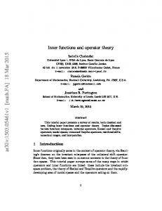
Figure 2.1.: Illustration of different belief function representations. The frame of discernment Θ consists of three elements a, b, c in this example and the triangle contains all subsets of Θ except for ∅. The indicated areas correspond to the mass of the different belief representations m, bel, pl, and q associated with the set {a, b}.

A = {a, b}, one abstains from making any statement about whether a is more “probable” than b. Instead, such an assignment expresses complete ignorance about this question. There are several equivalent representations for quantifying belief within the belief function framework. The four most important representations are mass functions denoted by m, belief functions denoted by bel, plausibility functions denoted by pl, and commonality functions denoted by q. An illustration of these representations is shown in Fig. 2.1. All these representations convey exactly the same information because they are in one-to-one correspondence to each other. The term “belief function” is somewhat ambiguous because it is used both as a general term (encompassing all the different representations) and as a specific term referring to the bel representation. In this work, the term is used in the general sense unless explicitly stated otherwise. The following sections introduce the different belief representations in a formal manner. In addition, rules for converting between the representations are defined as well as the most important classes of belief functions.

2.1.1. Mass Function A mass function (also called basic belief assignment or basic probability assignment) is in many respects the most fundamental belief representation and all other representations can be easily obtained from a mass function. Formally, a mass function m is a mapping m : P(Θ) → [0, 1] assigning a mass value to each

24

2.1. BELIEF FUNCTIONS hypothesis A ⊆ Θ of the frame of discernment Θ such that X m(A) = 1.

(2.2)

A⊆Θ

The value m(A) is the amount of belief strictly committed to hypothesis A. Such an assignment to a set A implies ignorance about the belief distribution over subsets of A. In Shafer’s original work [Shafer, 1976], there is an additional constraint requiring that a mass function must not assign a positive value to the empty set. m(∅) = 0 (2.3) A mass function satisfying this property is called normalized. This constraint is absent in the TBM framework where the mass assigned to ∅ usually represents the possibility that the true value is not included in the frame of discernment. Smets therefore argues that requiring m(∅) = 0 corresponds to a closed-world assumption while allowing m(∅) > 0 corresponds to an open-world assumption [Smets, 1992b, Smets, 1988]. All models presented in this work are based on a closed-world assumption. This means the frame of discernment is assumed to be exhaustive. As a result, belief functions are usually normalized. There are some exceptions where unnormalized belief functions are used (see Chap. 4). However, in this case, the use of unnormalized belief functions mainly serves as a way of explicitly representing conflict between different pieces of evidence. Regardless of the purpose, it is always possible to turn an unnormalized mass function m into a normalized mass function m0 . ( m(A) if A 6= ∅ (2.4) m0 (A) = 1−m(∅) 0 if A = ∅ Here, the factor (1 − m(∅))−1 acts as a normalization constant. Often, one is only interested in the sets A ⊆ Θ with positive mass values m(A) > 0. Such sets are called focal sets. The set Fm consisting of all focal sets corresponding to a mass function m is defined as Fm = {A|A ⊆ Θ, m(A) > 0}.

(2.5)

(Remark: Sets are generally denoted by capital letters while their elements are denoted by lower-case letters. For singletons, the bracket notation m({a}) can become quite cumbersome which is why set brackets are usually omitted for singletons: m(a) = m({a}) with a ∈ Θ.)

2.1.2. Belief Function The total amount of belief committed to a hypothesis A ⊆ Θ, including all subsets B ⊆ A, is denoted by bel(A). The function bel : P(Θ) → [0, 1] is called

25

CHAPTER 2. BELIEF FUNCTION THEORY a belief function (understood in the specific rather than in the general sense of the term). It can be directly computed from a mass function m. X

bel(A) =

∀A ⊆ Θ, A 6= ∅

m(B),

(2.6)

B⊆A,B6=∅

bel(∅) = 0

(2.7)

If m is normalized, a direct consequence of Eq. (2.6) is bel(Θ) = 1.

(2.8)

The property of subadditivity of a belief function bel was already defined in Eq. (2.1). The inequality bel(A) + bel(A) < 1 holds whenever there is a focal set B that is neither a subset of A nor of A (for example, if m(Θ) > 0 and A 6= Θ). A belief function bel is sometimes interpreted as defining a “lower bound” for an unknown probability function P , although this interpretation is only valid under specific circumstances (see Sect. 1.1). However, for a given belief function bel, one can always find a probability function P such that bel(A) ≤ P (A),

∀A ⊆ Θ.

(2.9)

In this case, bel and P are called compatible. When dealing with unnormalized mass functions, it is sometimes more convenient to use the so-called implicability function b instead of bel. The only difference is that it includes the mass assigned to the empty set. b(A) = bel(A) + m(∅) =

X

m(B),

∀A ⊆ Θ

(2.10)

B⊆A

Its interpretation is less intuitive though and it mostly serves a notational purpose. As stated above, all the different belief representations are in one-to-one correspondence. Just as it is possible to obtain a belief function bel from a mass function m using Eq. (2.6), it is also possible to recover a mass function from a belief function bel (or b if the beliefs are not normalized). This conversion is based on the Fast M¨obius Transformation [Thoma, 1989]. m(A) =

X

(−1)|A\B| b(B),

∀A ⊆ Θ

(2.11)

B⊆A

Such conversions are particularly useful if a certain representation simplifies the computations associated with an operation like evidence combination (see Sect. 2.2).

26

2.1. BELIEF FUNCTIONS

2.1.3. Plausibility Function The plausibility pl(A) is the amount of belief not strictly committed to the complement A. It therefore expresses how plausible a hypothesis A is, i.e., how much belief mass potentially supports A. On a formal level, a plausibility function pl : P(Θ) → [0, 1] is defined as pl(A) = bel(Θ) − bel(A),

∀A ⊆ Θ.

(2.12)

For the special case of normalized plausibility functions where bel(Θ) = 1, this definition reduces to ∀A ⊆ Θ.

pl(A) = 1 − bel(A),

(2.13)

The plausibility pl(A) can be computed from a mass function m in the following way: X pl(A) = m(B), ∀A ⊆ Θ, (2.14) B⊆Θ,B∩A6=∅

pl(∅) = 0.

(2.15)

Whereas bel can be viewed as a lower bound for an unknown probability function P under a lower- and upper probability interpretation, the plausibility can be viewed as an upper bound.1 For a normalized plausibility function pl, a compatible probability function P must satisfy the property pl(A) ≥ P (A),

∀A ⊆ Θ.

(2.16)

2.1.4. Commonality Function The commonality q(A) states how much mass in total is committed to A and all of the supersets B with A ⊆ B ⊆ Θ. The commonality q(A) therefore expresses how much mass potentially supports the entire set A. A commonality function q : P(Θ) → [0, 1] is defined as q(A) =

X

m(B),

∀A ⊆ Θ.

(2.17)

B⊆Θ,B⊇A

In order to compute a mass function m from a given commonality function q, the following equation can be used: X m(A) = (−1)|B\A| q(B), ∀A ⊆ Θ. (2.18) B⊆Θ,B⊇A 1

In fact, Shafer refers to pl as the “upper probability function” [Shafer, 1976, chapter 2].

27

CHAPTER 2. BELIEF FUNCTION THEORY

2.1.5. Classes of Belief Functions Regardless of the representation, there are certain classes of belief functions that are particularly important. These classes are defined in the following. Categorical Belief Function A belief function is called categorical if it is normalized and has only one focal set. m(A) = 1, A ⊆ Θ (2.19) Vacuous Belief Function A belief function is called vacuous if it is categorical and the focal set is the frame of discernment Θ. m(Θ) = 1 (2.20) A vacuous belief function represents a state of total ignorance. Simple Belief Function A simple belief function has at most two focal sets: the frame of discernment Θ and a strict subset of Θ. m(A) = 1 − w, m(Θ) = w

A ⊂ Θ, 0 ≤ w ≤ 1

(2.21) (2.22)

Dogmatic Belief Functions A belief function is called dogmatic if the frame of discernment Θ is not a focal set. m(Θ) = 0 (2.23) Consonant Belief Function A belief function is called consonant if its focal sets are nested. This means there exists an ordering of all the focal sets, such that A 0 ⊂ A 1 ⊂ . . . ⊂ Ak ,

with Ai ∈ Fm .

(2.24)

As a result, a consonant belief function only has up to |Θ| + 1 focal sets. The corresponding belief and plausibility functions satisfy the following properties [Shafer, 1976, chapter 10]: bel(A ∩ B) = min(bel(A), bel(B)), ∀A, B ⊆ Θ, pl(A ∪ B) = max(pl(A), pl(B)), ∀A, B ⊆ Θ.

(2.25) (2.26)

Note that the plausibility function defines a possibility measure in this case (see Sect. 5.4.5).

28

2.2. COMBINATION RULES Bayesian Belief Function A belief function is called Bayesian if it is normalized and all of its focal sets are singletons, i.e., if it is a probability function. In this case, the belief function bel satisfies the property of additivity defined by the Kolmogorov axioms [Kolmogorov, 1933]. bel(A ∪ B) = bel(A) + bel(B) if A ∩ B = ∅ with A, B ⊆ Θ

(2.27)

In addition, the following equalities hold for Bayesian belief functions: P (A) = bel(A) = pl(A), ∀A ⊆ Θ, P (a) = m(a) = q(a), ∀a ∈ Θ.

(2.28) (2.29)

2.2. Combination Rules In order to solve inference problems, belief functions representing different pieces of evidence need to be combined in a meaningful way. This is why combination rules are a major building block of belief function theory. Typically, each piece of evidence is represented by a separate belief function. Combination rules are then used to successively fuse all these belief functions in order to obtain a belief function representing all available evidence. There exist many different types of combination rules within the belief function framework. Surveys of different combination rules are given in [Smets, 2007] and [Sentz and Ferson, 2002]. The most important one is arguably Dempster’s rule. Most other combination rules are variations of Dempster’s rule and only differ in how they handle conflicting evidence. Generalizations of combination rules that can be parametrized are described in [Smets, 1997] and [Lefevre et al., 2002]. One of the reasons why new combination rules kept getting proposed over time was Zadeh’s criticism of Dempster’s rule when faced with highly conflicting evidence. In Zadeh’s example [Zadeh, 1979, Zadeh, 1984], two doctors independently diagnose the same patient, resulting in two (Bayesian) belief functions m1 and m2 where the frame of discernment {a, b, c} consists of three possible diseases. m1 (a) = 0.99 m2 (c) = 0.99

m1 (b) = 0.01 m2 (b) = 0.01

The result of combining these two belief functions using Dempster’s rule (see Sect. 2.2.1) is m(b) = 1, meaning that there is absolute certainty that the patient suffers from disease b. This was interpreted as being counterintuitive by some people because both doctors believe that b is highly unlikely. Combination rules handling this conflict in a different way are the conjunctive rule proposed by

29

CHAPTER 2. BELIEF FUNCTION THEORY Smets, Yager’s rule, and the rule proposed by Dubois and Prade. It should be noted that Zadeh’s criticism is not really limited to belief functions but can be used just as well against probability theory. The following sections introduce all combination rules used in this thesis. Dempster’s rule is the most important one because it is used throughout this work. The conjunctive and disjunctive rules are central elements in the TBM framework with the conjunctive rule being identical to Dempster’s rule apart from normalization. All other rules (Yager’s rule, Dubois and Prade’s rule, and the cautious rule) are only used in Chap. 4 where they are compared to Dempster’s rule and the conjunctive rule for a particular application.

2.2.1. Dempster’s Rule Dempster’s rule of combination was first introduced in [Dempster, 1967] and then reinterpreted by Shafer as a basis for belief function theory. It allows combining normalized belief functions that are defined over the same frame of discernment and are induced by “distinct bodies of evidence” (see Sect. 2.5 for a discussion of the notion of “distinctness”). The resulting belief function reflects a conjunctive combination of the underlying evidence. Let m1 and m2 be normalized mass functions induced by distinct pieces of evidence which are defined over the same frame of discernment Θ. The mass function m1⊕2 = m1 ⊕ m2 combined according to Dempster’s rule ⊕ is defined as X m1 (B) m2 (C), ∀A ⊆ Θ, A 6= ∅, (2.30) m1⊕2 (A) = η B∩C=A

m1⊕2 (∅) = 0, η −1 = 1 −

(2.31) X

m1 (B) m2 (C).

(2.32)

B∩C=∅

Here, η is a normalization constant assuring that the resulting mass function is normalized. It accounts for the products of mass values corresponding to all empty intersections of focal sets. Dempster’s rule is commutative, associative, and possesses a neutral element with the vacuous belief function. In contrast to most other rules, there exist a variety of theoretical justifications for the appropriateness of Dempster’s rule for combining evidence [Pichon and Denœux, 2010, Dubois and Prade, 1986a, Shafer and Tversky, 1985].2 In case there are more than two pieces of evidence, the corresponding belief functions are simply successively combined where the order of combination is irrelevant. When using normalized belief functions, a situation can occur in which two belief functions entirely contradict each other. This happens if all pairwise intersections of focal sets from the two mass functions are empty. In this case, 2

These justifications extend to the conjunctive rule which is almost identical.

30

2.2. COMBINATION RULES the belief functions are said to be flatly contradictory and their combination is undefined.3 The normalization constant η turns out to be more than just a nuisance because it represents the amount of conflict between two belief functions. The larger η becomes, the higher the conflict there is between m1 and m2 . Shafer defines the weight of conflict Con associated with the combination of two belief functions as the logarithm log(η) [Shafer, 1976, chapter 3]. X Con(m1 , m2 ) = − log(1 − m1 (B) m2 (C)) (2.33) B∩C=∅

The generalization to more than two belief functions is straightforward. The weight of conflict Con is 0 if there are no empty intersections of focal sets and it is infinite for flatly contradictory belief functions. In particular, the weight of conflict is additive. Con(m1 , . . . , mn+1 ) = Con(m1 , . . . , mn ) + Con(m1 ⊕ . . . ⊕ mn , mn+1 ) (2.34) Dempster’s rule is often interpreted as a generalization of Bayes’ rule. The reason for this interpretation becomes apparent when considering the combination of two Bayesian belief functions. Let e1 , e2 denote two pieces of evidence. By applying Bayes’ rule twice and assuming conditional independence between e1 , e2 given x, one has: P (x|e1 , e2 ) ∝ P (e1 |x) P (e2 |x) P (x) ∝

P (x|e1 ) P (x|e2 ) P (x). P (x) P (x)

(2.35)

Ignoring the prior P (x) at the very end (the prior constitutes a separate piece of evidence in the belief function framework), this product corresponds to a special case of Dempster’s rule. By setting mi (x) ∝ P (x|ei )/P (x), each mass function mi represents the (prior-free) belief induced by evidence ei . In this case, the combination m1 ⊕ m2 is equal to the posterior probability distribution P (x|e1 , e2 ). Although in most cases Dempster’s rule is applied to mass functions, commonality functions are actually a more convenient form of representation for Dempster’s rule. Let q1 , q2 be the commonality functions corresponding to the mass functions m1 , m2 and let q1⊕2 be the commonality function corresponding to the mass function m1 ⊕ m2 . Dempster’s rule can then be expressed in the following way: q1⊕2 (A) = η q1 (A) q2 (A), ∀A ⊆ Θ, A 6= ∅ q1⊕2 (∅) = 1 X η −1 = (−1)|B|+1 q1 (B) q2 (B)

(2.36) (2.37) (2.38)

B⊆Θ,B6=∅ 3

The same can happen with probability functions when applying the Bayesian theorem if all prior-likelihood products are 0.

31

CHAPTER 2. BELIEF FUNCTION THEORY It turns out that for commonality functions, Dempster’s rule of combination reduces to computing a simple product of commonality values where η is a normalization constant equal to the one defined in Eq. (2.32). Such a product can be computed more efficiently than the expression in Eq. (2.30). The question in this case is whether a potential conversion to commonalities is worth the reduced computational effort of the combination.

2.2.2. Conjunctive Rule The conjunctive rule of combination is an adaptation of Dempster’s rule and plays a central role in the TBM framework [Smets and Kennes, 1994]. Because the TBM framework explicitly allows unnormalized belief functions, the normalization step performed by Dempster’s rule is omitted. Otherwise it is identical to Dempster’s rule. Let m1 and m2 be two (possibly unnormalized) mass functions induced by distinct pieces of evidence and which are defined over the same frame of discernment Θ. The mass function m1 ∩ m2 resulting from the combination ∩ 2 = m1 using the conjunctive rule ∩ is defined as X m1 (A) = m1 (B) m2 (C), ∀A ⊆ Θ. (2.39) ∩2 B∩C=A

Other than for Dempster’s rule, the result of the conjunctive rule of combination is always defined. For flatly contradictory evidence, the result is simply m1 ∩ 2 (∅) = 1. Just like Dempster’s rule can be efficiently computed in terms of commonality functions, the same applies to the conjunctive rule. Let q1 , q2 , and q1 ∩ 2 be the commonality functions corresponding to the mass functions m1 , m2 , and m1 ∩2 respectively. Then the conjunctive combination of q1 and q2 is defined as q1 ∩ 2 (A) = q1 (A) q2 (A),

∀A ⊆ Θ.

(2.40)

As discussed in Sect. 2.1.1, the question whether normalization should be performed usually depends on whether one makes an open- or a closed-world assumption. Under an open-world assumption, normalization should not be performed and the conjunctive rule of combination should be used instead of Dempster’s rule. Under a closed-world assumption, the need for normalization depends on the application. On the one hand, a positive mass value m(∅) provides useful information even for a closed-world assumption. This is because the conflict between the underlying pieces of evidence is described by the mass on ∅ with Con(m1 , m2 ) = − log(1 − m1 ∩ 2 (∅)). In contrast to Dempster’s rule, this conflict information is preserved when performing multiple combinations even if the original belief functions are not available anymore. If such information is useful for an application (e.g., see Chap. 4), normalization should be avoided. On the other hand, if one is not interested in the amount of conflict, normalization should be performed and Dempster’s rule is more appropriate. In

32

2.2. COMBINATION RULES particular, normalization should be performed if there is significant conflict and belief functions are combined recursively over time. An example of such a situation is the particle filter presented in Chap. 3, where omitting normalization would cause m(∅) to quickly dominate all other mass values, meaning almost all particles would represent ∅.

2.2.3. Disjunctive Rule The disjunctive rule of combination [Dubois and Prade, 1986b] is applied when only one of several pieces of evidence holds. Whereas Dempster’s rule and the conjunctive rule correspond to an “and”-like operation, the disjunctive combination rule represents an “or”-like operation. However, the main use of the disjunctive rule is in the context of conditional belief functions, see Sect. 2.4. Let m1 and m2 be two (possibly unnormalized) mass functions induced by distinct pieces of evidence which are defined over the same frame of discernment Θ. The mass function m1 ∪ m2 resulting from the combination using ∪ 2 = m1 the disjunctive rule ∪ is defined as X (m1 ∪ m2 ) (A) = m1 (B) m2 (C), ∀A ⊆ Θ. (2.41) B∪C=A

Because the union B ∪ C is never empty unless both focal sets are empty, there is no conflict resulting from the disjunctive rule of combination and therefore no need for normalization. Just like commonality functions can be used for efficiently computing Dempster’s rule/the conjunctive rule, implicability functions can be used to express the disjunctive rule in terms of a simple product. Let b1 , b2 be the implicability functions corresponding to the mass functions m1 , m2 and let b1 ∪ 2 be the implicability function corresponding to the mass function m1 ∪ m2 . The disjunctive rule of combination is then defined as the product b1 ∪ 2 (A) = b1 (A) b2 (A),

∀A ⊆ Θ.

(2.42)

2.2.4. Other Rules Yager’s Rule In [Yager, 1987], Yager proposes a combination rule that assigns the mass associated with conflicting focal sets to the frame of discernment (instead of performing normalization or assigning it to ∅). Let m12 denote the result of combining two mass functions m1 , m2 induced by distinct pieces of evidence using Yager’s rule. Expressed in terms of the conjunctive rule, Yager’s rule is defined as   ∀A ⊂ Θ, A 6= ∅, ∩ 2 (A) m1 m12 (A) = m1 (2.43) if A = Θ, ∩ 2 (Θ) + m1 ∩ 2 (∅)   0 if A = ∅.

33

CHAPTER 2. BELIEF FUNCTION THEORY This means that highly conflicting evidence leads to a state of high ignorance with all conflict-related mass m1 ∩ 2 (∅) being assigned to Θ. Dubois and Prade’s Rule The rule proposed by Dubois and Prade in [Dubois and Prade, 1986b] is similar to Yager’s rule. However, instead of assigning the mass of conflicting focal sets to the frame of discernment, it is assigned to the union of the corresponding focal sets. Let m12 denote the result of combining two mass functions m1 , m2 induced by distinct pieces of evidence using Dubois and Prade’s rule. Expressed using the conjunctive rule of combination, the rule is defined as ( P m1 ∩ 2 (A)+ B∩C=∅,B∪C=A m1 (B) m2 (C) ∀A ⊆ Θ, A 6= ∅, m12 (A) = (2.44) 0 if A = ∅. Note that for |Θ| = 2, Yager’s rule and Dubois and Prade’s rule are identical. Cautious Rule The cautious combination rule was introduced in [Denœux, 2008] and differs significantly from all the other rules presented here. Whereas the other rules all assume that the underlying pieces of evidence are “distinct”, the cautious rule allows combining non-distinct/overlapping pieces of evidence. The rule shown below is also referred to as the “cautious conjunctive rule” because there also exists a disjunctive version that is not considered here. Before defining the actual combination rule, some additional concepts and notation need to be introduced. Let Aw denote the simple belief function defined by m(A) = 1 − w and m(Θ) = w. In [Smets, 1995], it is shown that any non-dogmatic belief function can be uniquely represented as a conjunctive combination of simple belief functions Aw(A) with w(A) m= ∩ A⊂Θ A , Y |B|−|A|+1 w(A) = q(B)−1 ,

(2.45) ∀A ⊂ Θ,

(2.46)

B⊇A

where w(A) : P(Θ) \ Θ → [0, +∞] is a weight function that can be computed using the commonality function q belonging to mass function m. Let m1 , m2 be two non-dogmatic mass functions (possibly induced by nondistinct pieces of evidence). Let w1 , w2 be the corresponding weight functions and let m12 denote the result of combining m1 with m2 using the cautious rule. min(w1 (A),w2 (A)) m12 = ∩ A⊆Θ A

(2.47)

The cautious rule is thus computed in terms of a combined weight function A 7→ min(w1 (A), w2 (A)) where the min-operator corresponds to a conjunctive combination of w1 and w2 .

34

2.3. EXTENSION AND MARGINALIZATION

2.3. Extension and Marginalization When combining two belief functions that are defined over different frames of discernment, both first need to be extended to the joint space. Let Θ1 , Θ2 be the non-overlapping frames of discernment of mass functions m1 , m2 respectively. The combination of m1 and m2 using, for example, Dempster’s rule is then defined over the joint frame of discernment Θ1 × Θ2 . The respective extensions of m1 and m2 required prior to this combination are defined as 1 ×Θ2 (A × Θ2 ) = m1 (A), m↑Θ 1

∀A ⊆ Θ1 ,

(2.48)

1 ×Θ2 (Θ1 m↑Θ 2

∀B ⊆ Θ2 .

(2.49)

× B) = m2 (B),

In order to keep notation simple, extensions are omitted throughout the text whenever possible and combined mass functions are implicitly assumed to be defined over their respective joint space. This also means that whenever set operations are performed over a joint space, the operands are implicitly assumed to be extended first (e.g., A ∩ B with A ⊆ Θ1 , B ⊆ Θ2 actually means (A × Θ2 ) ∩ (Θ1 × B)). Furthermore, the notation A, B is used to denote A ∩ B. Conversely to extension, a belief function defined over some joint frame of discernment can be marginalized. Let mass function m12 be defined over Θ1 ×Θ2 . ↓Θ2 1 The marginal mass functions m↓Θ 12 and m12 defined over Θ1 and Θ2 respectively are defined as X 1 m↓Θ (A) = m12 (A × B), ∀A ⊆ Θ1 , (2.50) 12 B⊆Θ2 2 m↓Θ 12 (B) =

X

m12 (A × B),

∀B ⊆ Θ2 .

(2.51)

A⊆Θ1

Just like extension is usually omitted for notational simplicity, marginalization is omitted as well. The extension defined in Eq. (2.48) and (2.49) is also referred to as a vacuous extension because marginalizing on the “newly added space” always yields a vacuous belief function: 1 ×Θ2 ↓Θ2 m↑Θ (Θ2 ) = 1, 1

(2.52)

1 ×Θ2 ↓Θ1 m↑Θ (Θ1 ) = 1. 2

(2.53)

2.4. Conditional Belief Functions Like probability functions, belief functions can be conditioned. If a subset A ⊂ Θ of the frame of discernment is known to be true with absolute certainty, then this fact can be expressed using the categorical mass function mA (A) = 1. Let m denote the mass function describing the belief prior to learning that subset

35

CHAPTER 2. BELIEF FUNCTION THEORY A is true. This prior belief can be conditioned with A by combining m with mA using Dempster’s rule4 , which results in the conditional mass function m[A]: m[A] = m ⊕ mA with mA (A) = 1.

(2.54)

(Remark: Writing m[A] opposed to m(·|A) has become the standard notation for conditional belief functions because operations often require the entire function as input. For example, it simplifies the notation for combinations where one can write m[A] ⊕ m[B] instead of m(·|A) ⊕ m(·|B).) Plugging in the definition of Dempster’s rule given by Eq. (2.30) yields the following expression for m[A]: ( P η C⊆A m(B ∪ C) ∀B ⊆ A, B 6= ∅, (2.55) m[A](B) = 0 otherwise, η = pl(A)−1 .

(2.56)

Eq. (2.55) is referred to as Dempster’s rule of conditioning. The corresponding plausibility function pl[A] is given by pl[A](B) =

pl(A ∩ B) , pl(A)

∀B ⊆ Θ.

(2.57)

Usually, when dealing with conditional belief functions m[A](B), A and B belong to different frames of discernment. In this case, extension and marginalization are implicitly assumed such that m[A](B) is a belief function defined over the frame of discernment corresponding to B. Conditional belief functions can also be used to make evidence explicit in the notation. Given some piece of evidence e, the induced mass function can be written as m[e]. As a result, a combination of two pieces of evidence e1 , e2 based on a rule ~ with ~ ∈ {⊕, ∩, ∪ , . . .} can be written with the evidence made explicit: m[e1 , e2 ] = m[e1 ] ~ m[e2 ]. (2.58) Assuming one has a set of belief functions with frame of discernment Θ, each conditioned by an element from a different frame of discernment Ω, the disjunctive rule of combination allows one to construct a belief function conditioned by an arbitrary subset of Ω. This is very useful in practice because one oftentimes is only provided with singleton-conditioned belief functions when, instead, one needs a belief function conditioned by a larger set. Let {f [ai ]|1 ≤ i ≤ k} be a set of conditional belief functions defined over Θ with f ∈ {m, bel, pl, q} and ai ∈ Ω. If the evidence underlying each belief function f [ai ] is distinct, the disjunctive rule of combination can then be used to construct the belief function f [A] with A ⊆ Ω [Smets, 1993]: ∪ f [ai ], f [A] = ○

∀A ⊆ Ω, A 6= ∅

(2.59)

ai ∈A 4

If unnormalized belief functions are allowed, the conjunctive rule should be used instead.

36

2.5. DISTINCTNESS AND INDEPENDENCE Using the disjunctive rule for combining the belief functions f [ai ] in Eq. (2.59) makes sense because A is a union of singletons ai , meaning that at least one element ai must hold if A holds. For mass, belief, and plausibility functions, disjunctively combining such singleton-induced belief functions results in the following equations [Smets, 1993]: X

m[A](B) = (

S

Y

Bi )=B

m[ai ](Bi ),

(2.60)

ai ∈A

i:ai ∈A

bel[A](B) =

Y

bel[ai ](B),

(2.61)

Y

(2.62)

ai ∈A

pl[A](B) = 1 −

(1 − pl[ai ](B)).

ai ∈A

Another important use of conditional belief functions is that they can sometimes simplify the computation of Dempster’s rule of combination. In case it is easier to express a belief function in a conditional form, Dempster’s rule for combining two belief functions defined over Θ can be stated in a different way. If f1 is a normalized belief function with f ∈ {m, bel, pl, q} and m2 is a normalized mass function, then the combination f1⊕2 according to Dempster’s rule can be computed by [Dubois and Prade, 1986a] f1⊕2 (A) = η

X

f1∗ [B](A) m2 (B) ∀A ⊆ Θ,

(2.63)

B⊆Θ,B6=∅

f1∗ [B](A) = f1 [B](A) pl1 (B).

(2.64)

Eq. (2.63) is essentially a generalization of the law of total probability. It is therefore referred to as the f -total law and it turns out to be very useful in practice. Note that the conditioning of f1 with B is generally unnormalized (bel1∗ [B](Θ) ≤ 1), making the notation a little cumbersome if the final outcome is supposed to be normalized. Because conditional belief functions are defined in terms of Dempster’s rule in Eq. (2.54), the associated normalization has to be undone in Eq. (2.64) by multiplying with the normalization constant pl1 (B) introduced in Eq. (2.56) [Smets, 1991]. There are two important cases in which this “denormalization” can be omitted: (i) if all involved belief functions are ∗ unnormalized and f1 ∩ 2 is computed instead of f1⊕2 or (ii) if f1 [B] is normalized for any B, which is the case if A and B are defined over different frames of discernment.

2.5. Distinctness and Independence All combination rules presented in Sect. 2.2 require the underlying pieces of evidence to be “distinct” (except for the cautious rule). Unfortunately, the notion

37

CHAPTER 2. BELIEF FUNCTION THEORY of distinctness was never defined in a formal way for non-Dempsterian interpretations of belief functions [Shafer and Tversky, 1985]. A detailed discussion of this problem can be found in [Smets, 1992a]. For the special case of Bayesian belief functions, distinctness reduces to probabilistic conditional independence, which can be seen in Eq. (2.35) [Smets, 2007]. For general belief functions, the following definition, which works well in practice and is shared by many works, is adopted (e.g., [Smets, 1998b]): Definition. Two pieces of evidence e1 , e2 are said to be distinct if and only if learning that e2 is true does not influence the belief induced by e1 and vice versa. Regarding the combination process, this essentially means that no piece of evidence should be counted twice. When considering multiple variables, the notion of distinctness is usually not sufficient. In [Ben Yaghlane et al., 2002a] and [Ben Yaghlane et al., 2002b], the case of multiple variables is considered and the concepts of irrelevance and non-interactivity are introduced. Let X, Y be two evidential variables with frames of discernment ΘX , ΘY and let fΘX be a belief function over ΘX with fΘX ∈ {m, bel, pl, q}. Variable Y is said to be irrelevant with respect to X if and only if fΘX [Y ] = fΘX ,

∀Y ⊆ ΘY .

(2.65)

The concept of irrelevance is similar to distinctness because Y does not influence the belief in X and vice versa. In particular, irrelevance is a property that can usually be defined by an expert. In contrast, the concept of non-interactivity concerns the decomposability of belief functions. Variables X and Y are said to be non-interactive if and only if the joint belief function mΘX ×ΘY can be constructed from the marginal belief functions over ΘX and ΘY using Dempster’s rule.5 mΘX ×ΘY = mΘX ⊕ mΘY

(2.66)

For the conditional case with an additional variable Z, non-interactivity of X and Y given z with z ∈ ΘZ is defined as mΘX ×ΘY [z] = mΘX [z] ⊕ mΘY [z],

∀z ∈ ΘZ .

(2.67)

Non-interactivity implies irrelevance though the opposite is not generally true because non-interactivity additionally requires the preservation of irrelevance under Dempster’s rule [Ben Yaghlane et al., 2002a]. The concepts of irrelevance and non-interactivity are equivalent in probability theory where both reduce to the notion of conditional independence. 5

For unnormalized belief functions, non-interactivity can be defined in terms of the conjunctive rule, though in this case, an additional normalization constant is required [Ben Yaghlane et al., 2002b].

38

2.6. GENERALIZED BAYESIAN THEOREM Non-interactivity is equivalent to the concept of evidential independence introduced in [Shafer, 1976, chapter 7]. In the same work, the weaker notion of cognitive independence is also introduced. Evidential independence implies cognitive independence but not vice versa. Variables X and Y are said to be cognitively independent if and only if the joint plausibility function pl(X, Y ) can be factorized into the marginal plausibility functions pl(X) and pl(Y ). pl(X, Y ) = pl(X) pl(Y ),

∀X ⊆ ΘX , Y ⊆ ΘY .

(2.68)

If there is a third variable Z, variables X and Y are said to be conditionally cognitive independent given z if and only if [Smets, 1993] ∀X ⊆ ΘX , ∀Y ⊆ ΘY , z ∈ ΘZ .

pl[z](X, Y ) = pl[z](X) pl[z](Y ),

(2.69)

Note that for cases where the distinction between non-interactivity, irrelevance, and cognitive independence is not essential, the more-common term “conditional independence” is usually used.

2.6. Generalized Bayesian Theorem The introduction of the generalized Bayesian theorem by Smets in [Smets, 1993] marks one of the major theoretical results for belief function theory. Without it, belief function theory could hardly be considered a generalization of Bayesian probability theory because there would be no way of handling likelihoods. Let X and Y be evidential variables with separate frames of discernment ΘX and ΘY . Like the name “generalized Bayesian theorem” suggests, it allows constructing a belief function over ΘX from belief functions over ΘY conditioned on elements from ΘX . Let the singleton-conditioned plausibilities pl[x](Y ) with x ∈ ΘX , Y ⊆ ΘY be all the information that is available (pl[x](Y ) is referred to as the likelihood of x). Assuming each pl[x](Y ) results from distinct evidence, the belief function over ΘX can then be computed in the following way (the equation for m[Y ](X) is given in [Delmotte and Smets, 2004], all others can be found in [Smets, 1993]): Y Y (1 − pl[x](Y )), (2.70) m[Y ](X) = η pl[x](Y ) x∈X

bel[Y ](X) = η

Y

x∈X

bel[x](Y ) − η

Y

bel[x](Y ),

(2.71)

x∈ΘX

x∈X

pl[Y ](X) = η (1 −

Y

(1 − pl[x](Y ))),

(2.72)

x∈X

q[Y ](X) = η

Y

pl[x](Y ),

(2.73)

x∈X

η −1 = 1 −

Y

(1 − pl[x](Y )),

(2.74)

x∈ΘX

∀X ⊆ ΘX , Y ⊆ ΘY , X 6= ∅, Y 6= ∅.

39

CHAPTER 2. BELIEF FUNCTION THEORY These are the normalized versions of the generalized Bayesian theorem. For the unnormalized versions, the normalization constant η is simply omitted. Note that there is no prior over ΘX in these equations like in the classical Bayesian theorem. Thus, if a prior is not available, it can be ignored (which is not possible with the classical Bayesian theorem). However, in case there is a prior, it is combined with the resulting belief function using Dempster’s rule (or the conjunctive rule, depending on whether normalization is desired). Let e0 denote prior evidence inducing a belief over ΘX and let mΘX [Y ] denote the belief function computed from pl[x](Y ) according to Eq. (2.70). The belief function mΘX [Y, e0 ] reflecting all the available evidence is then given by mΘX [Y, e0 ] = mΘX [Y ] ⊕ mΘX [e0 ].

(2.75)

The generalized Bayesian theorem is particularly useful if there is a variable X representing a “cause” and a set of variables Yi with 1 ≤ i ≤ n representing various “effects”. Just like the classical Bayesian theorem, the generalized Bayesian theorem allows computing the belief over possible causes given the observed effects. In order for the generalized Bayesian theorem to be applicable, the distributions pl[x](Y1:n ) over the effects need to be independent from each other for each context x ∈ ΘX . If furthermore conditional cognitive independence holds between the effects given a common cause, then each cause-effect relation can be described by a separate model pl[x](Yi ). The belief over X can then simply be computed from a set of observed effects y1:n using Eq. (2.70) where the joint effect plausibility is factorized due to conditional cognitive independence. Y Y (2.70) (1 − pl[x](y1:n )) (2.76) m[y1:n ](X) = η pl[x](y1:n ) x∈X (2.69)

= η

n YY

x∈X

pl[x](yi )

x∈X i=1

Y

(1 −

x∈X

n Y

pl[x](yi ))

(2.77)

i=1

Note that this is equivalent to independently computing the belief mΘX [yi ] for each observation yi using Eq. (2.70) and then combining the belief functions using Dempster’s rule [Smets, 1993]). mΘX [y1:n ] =

n M

mΘX [yi ]

(2.78)

i=1

The name “generalized Bayesian theorem” stems from the fact that it reduces to the classical Bayesian theorem if the conditional plausibilities are probability functions and if there is furthermore a Bayesian prior over ΘX . By assuming pl[x](y) = P (y|x) and m[e0 ](x) = P (x) where e0 represents the prior evidence for x, the classical Bayesian theorem for the posterior P (x|y) can be recovered in the following way (the right hand side shows the respective equations required for each transformation):

40

2.7. PIGNISTIC TRANSFORMATION

P (x|y) = q[y, e0 ](x) ∝ q[y](x) q[e0 ](x) ∝ pl[x](y) q[e0 ](x) = P (y|x) P (x)

(Eq. (2.29)) (Eq. (2.75) and (2.36)) (Eq. (2.73)) (assumption)

(2.79) (2.80) (2.81) (2.82)

2.7. Pignistic Transformation In order to make decisions based on belief functions, Smets argues that beliefs first need to be transformed to probabilities [Smets, 2005b, Smets, 2002]. This reflects the distinction between the credal and the pignistic level within the TBM framework where the pignistic level is used for decision making. Only at the pignistic level is it possible to compute an expected value of a utility function, which is the basis for rational decision making. Transforming a belief function into a pignistic probability function is done via the pignistic transformation. Let m denote a mass function with frame of discernment Θ and let BetPm denote the corresponding pignistic probability function. The pignistic transformation of m into BetPm is defined as BetPm (a) =

m(A) , |A| (1 − m(∅)) A3a

X

∀a ∈ Θ.

(2.83)

The normalization constant 1 − m(∅) can be omitted if m is normalized. Essentially, this transformation causes all mass values assigned to focal sets A with |A| > 1 to be evenly distributed among the elements a ∈ A. For example, a vacuous belief function would be transformed into a uniform probability distribution. (Remark: If a piece of evidence e induces a belief function m[e], the notation BetP [e] is used to denote the pignistic transformation of m[e].) The pignistic transformation can be used to compute the expected value of a real-valued random variable. Let X be a random variable mapping elements from the finite set Θ to the reals R. Let BetPm be the pignistic transformation of a mass function m defined over Θ. The expected value E(X) is then defined as [Smets, 2005b] X X(θ) BetPm (θ). (2.84) E(X) = θ∈Θ

2.8. Uncertainty Measures Both on theoretical and practical grounds, being able to quantify the amount of uncertainty associated with a belief function is useful. For example, in Chap. 5,

41

CHAPTER 2. BELIEF FUNCTION THEORY a system is presented which actively seeks to minimize uncertainty by selecting actions with the highest expected information gain. Because this system is based on belief functions, it requires a way of measuring the amount of uncertainty associated with a belief function. For probability functions, the Shannon entropy [Shannon, 1948] constitutes a commonly accepted measure of uncertainty. Let P denote the probability function associated with a discrete random variable X defined over the sample space Θ. The Shannon entropy H is defined as the expected value of the selfinformation − logb P (x) of each event x ∈ Θ. X H(P ) = − P (x) logb P (x) (2.85) x∈Θ

Because information is usually measured in bits, b = 2 is the most common choice. In case there is no uncertainty (P (x) = 1 for some x ∈ Θ), the Shannon entropy is 0. The Shannon entropy increases the more uniform the distribution P becomes and it reaches its maximum for an entirely uniform distribution, which represents a state of total uncertainty in the Bayesian framework. Unfortunately, there is no commonly accepted measure of uncertainty for general belief functions, despite many attempts to generalize the concept of Shannon entropy (see [Klir and Smith, 2001, Klir, 2004, Klir, 1999, Pal et al., 1992] for overviews). For belief functions, there are two kinds of uncertainty: nonspecificity and conflict.6 Non-specificity (also called ignorance) refers to the fact that hypotheses are sets with arbitrary cardinality and thus carry uncertainty in themselves (which element in a focal set is true?). This kind of uncertainty is captured by Hartley’s measure of non-specificity HL [Hartley, 1928], which quantifies the uncertainty of a focal set in terms of its cardinality. The generalized Hartley measure GH [Klir, 2005] quantifies the overall amount of non-specificity associated with a mass function m. HL(A) = logb |A| X GH(m) = m(A) logb |A|

(2.86) (2.87)

A∈Fm

In contrast, conflict is the uncertainty found in classical probability theory with mutually exclusive (i.e., conflicting) events and it is adequately captured by the Shannon entropy. An uncertainty measure for belief functions should satisfy a number of requirements [Klir, 2005] and it should reflect both non-specificity and conflict. Up to this point, only one measure satisfying all the desired requirements has been found (most measures fail to satisfy the property of sub-additivity). This measure is called Aggregate Uncertainty (AU ). Let f be a belief function with 6

Not to be confused with the conflict between different belief function as measured by the weight of conflict Con.

42

2.8. UNCERTAINTY MEASURES f ∈ {m, bel, pl, q}, then AU is defined as the maximum Shannon entropy over the set P(f ) of all probability functions compatible (see Eq. (2.9)) with f . AU (f ) = max H(P ) P ∈P(f )

(2.88)

The measure’s name results from the fact that it captures non-specificity and conflict in an aggregated fashion. Furthermore, it reduces to Shannon entropy for the special case of a Bayesian belief function. Even though computing the AU measure requires finding the solution to a non-linear optimization problem, there exists an “efficient” algorithm with worst-case time complexity O(|P(Θ)|2 ) where Θ denotes the frame of discernment of f [Harmanec, 1997]. It should be noted that AU is also an appealing solution in the context of other uncertainty frameworks (e.g., possibility theory). However, there are also a number of problems with the AU measure. First, it is insensitive to strong belief changes because of the max operation (see [Klir, 2004] for an example). Second, despite the availability of an efficient algorithm, it is computationally expensive, which is particularly problematic if it has to be computed many times. Third, its adequacy is questionable when belief functions are not interpreted as defining lower and upper probability bounds. For these reasons (in particular the first two), the AU measure is not used in this work. Instead, a simpler measure based on the pignistic transformation is proposed, which is referred to here as pignistic entropy [Reineking, 2008]. Like the name suggests, the pignistic entropy HBetP is computed by first applying the pignistic transformation to a belief function and then computing the Shannon entropy of the resulting probability distribution. The pignistic entropy of a mass function m is defined as HBetP (m) = H(BetPm ).

(2.89)

This measure is justified in particular in a classification context where the pignistic transformation is applied in order to determine the most probable class (which is the case in Chap. 5). In addition, it can be computed much more efficiently with worst-case time complexity O(|P(Θ)|), which is a result of computing the pignistic transformation.

43

3

Evidential Particle Filtering 3.1. Introduction In this chapter, a particle filter algorithm is derived within the belief function framework. The main results presented in this chapter were originally proposed in [Reineking, 2011]. Some preliminary work regarding the temporal updating of belief functions was presented in [Reineking, 2008]. Particle filtering is one of the most widely-applied probabilistic techniques for estimating the state of a dynamical system where state transitions and observations are subject to uncertainty [Doucet et al., 2001]. Being a Monte-Carlo approach, a finite number of samples (or particles) is used to approximate the probability (density) distribution of the current state. The state is usually described by a low-dimensional vector because the number of samples required for accurately approximating the underlying distribution tends to grow exponentially with the number of dimensions. Especially in robotics, particle filters have been extremely successful for problems like localization [Thrun et al., 2001] and SLAM [Montemerlo et al., 2002], but they are also commonly used in other domains like computer vision [Isard and Blake, 1998]. Compared to Kalman filters [Kalman, 1960], the most popular alternative approach for state estimation, particle filters provide a number of important advantages. In Kalman filters, the distribution of the current state is modeled as a Gaussian and both state transitions and observations are modeled as linear functions with additive Gaussian noise. While the linearity requirement can be relaxed (using extended or unscented Kalman filters [Ljung, 1979, Wan and van der Merwe, 2000]), the class of distributions that can be expressed using Kalman filters is much more restricted compared to particle filters. In particular, particle filters are able to handle multi-modal distributions well and can

45

CHAPTER 3. EVIDENTIAL PARTICLE FILTERING also be applied to discrete state variables. Because of these reasons, particle filters have become the standard solution for estimation problems in many domains. For situations where the state prior, transitions, or observations can be more accurately described by belief functions opposed to probability functions, being able to perform particle filtering based on belief functions would be very useful. The approach presented in this chapter does exactly this by generalizing the concept of particle filtering in the belief function framework. The two major contributions of the work presented in this chapter are: • Derivation of recursive update equations based on belief functions which generalize Bayesian filtering. • Efficient approximations of the solutions to these equations based on an evidential particle filter algorithm. The belief about the current state, transitions, and observations are all described by belief functions in this case, allowing the use of richer uncertainty models capable of expressing partial or total ignorance when appropriate. In order to make the computations tractable, the belief about the current state is approximated by a finite number of samples. This reduces the exponential complexity of the exact solution to a complexity which is linear with respect to the size of the state space. It should be noted that, throughout this chapter, the state is assumed to be a discrete variable. In contrast, observations can be discrete or continuous (handling continuous measurements is described in [Smets, 2005a]). A discussion of extending the presented approach to continuous state variables can be found at the end of the chapter. The remainder of this chapter is structured as follows. The next section provides a brief overview of related work. In Sect. 3.3, a belief function filter and its recursive update equations are derived. An evidential particle filter algorithm, a Monte-Carlo solution to the update equations, is presented in Sect. 3.4 along with a detailed derivation. The computational complexity of the algorithm and the corresponding approximation error are analyzed in Sect. 3.5. In Sect. 3.6, the algorithm is applied to a bearings-only tracking problem where the tracking error of the evidential solution is compared to the performance of a corresponding probabilistic solution. In the final section, the presented approach and possible extensions are discussed.

3.2. Related Work The work related to the approach presented in this chapter can be roughly divided into two areas. The first is concerned with modeling temporal processes using belief functions. The second is concerned with Monte-Carlo approaches for efficiently combining belief functions.

46

3.2. RELATED WORK

3.2.1. Temporal Updating of Belief Functions In the context of filtering based on belief functions, a solution to the problem of joint tracking and classification in the TBM framework is proposed in [Smets and Ristic, 2007, Smets and Ristic, 2004]. The authors derive a Kalman filter algorithm where the underlying belief functions are implicitly represented by their pignistic transformations which are Gaussians. The evidential Kalman filter is used to track an object and estimate its class based on the observed motion behavior. Due to the evidential representation, it is possible to dissociate the motion behavior from the class, resulting in a higher classification accuracy compared to a Bayesian solution. There are several works about filtering based on probabilistic dynamics and evidential processing of observations. In [Mu˜ noz-Salinas et al., 2009], a person is tracked by multiple cameras where belief functions are used to handle the problem of the person being out of sight. Similarly, in [Klein et al., 2010], a particle filter performs visual tracking and different belief function combination rules are used to fuse information sources based on their reliability and precision. In [Ramasso et al., 2007a], hidden Markov models are generalized within the TBM framework. Beliefs are represented by commonality functions here which simplifies some of the computations. Among other things, an evidential version of the Viterbi algorithm is proposed and an application to human motion analysis is described (cf. [Ramasso et al., 2007b]).

3.2.2. Monte-Carlo Approximations of Belief Functions When dealing with large frames of discernment, exact belief function inference becomes infeasible and approximate approaches are required. The use of Monte-Carlo methods is an obvious choice in this case, which is why several sampling-based inference approaches for belief functions have been proposed over time [Wilson, 2000, Moral and Wilson, 1996, Moral and Salmer´on, 1999, Kreinovich et al., 1994]. Despite the success of Monte-Carlo approaches in many fields, their overall popularity in the context of belief function theory is still limited. Most Monte-Carlo approaches for belief functions aim to approximate the belief resulting from combining two or more belief functions using Dempster’s rule of combination. For Dempster’s rule, the normalization is particularly problematic with respect to sampling. Without normalization (e.g., for the conjunctive rule of combination) or when conflict is low, a simple Monte-Carlo algorithm could independently draw samples from each mass function and build the intersection of these samples. However, for highly conflicting belief functions, most intersections would be empty and thus invalid if no mass on ∅ is allowed. Therefore, such a simple Monte-Carlo algorithm would either yield poor approximations (with few valid samples) or it would be very inefficient (when repeating the sampling process until enough non-empty intersections are found).

47

CHAPTER 3. EVIDENTIAL PARTICLE FILTERING For this reason, two Monte-Carlo methods have been proposed which are able to handle highly conflicting evidence when approximating Dempster’s rule. The first method is based on Markov chain Monte-Carlo [Wilson and Moral, 1996] where a Markov chain is used in order to draw samples from the underlying belief distribution. While yielding good approximations, this method is not suited for particle filtering because it requires multiple runs in order to produce accurate results, which is not acceptable for an online particle filter algorithm. The second method is importance sampling [Moral and Wilson, 1996]. Here, samples are drawn from a different distribution (i.e., one which makes empty intersections impossible), and importance weights are used to account for the difference between the true distribution and the sampled one. A detailed description of importance sampling is given in Sect. 3.4.2. Note that importance sampling is also used in most probabilistic particle filter algorithms.

3.3. Evidential Filtering In this section, the equations for filtering based on belief functions are derived. In addition, it is shown that these equations reduce to Bayesian filtering [Thrun et al., 2005, chapter 2] if the prior and the underlying transition and observation models are Bayesian belief functions. Let Θt denote the discrete state space for state xt ∈ Θt at time t.1 Let Ωt denote the discrete or real-valued observation space for observation zt ∈ Ωt at time t (e.g., zt could be a sensor measurement). Let z0:t denote the sequence of all observations obtained over time (short for z0 , . . . , zt ). Without a loss of generality, it is assumed that state transitions and observations occur in alternating order, i.e., after each state transition from xt−1 to xt , an observation zt is recorded. This corresponds to the dynamic belief network shown in Fig. 3.1 (belief networks are a generalization of Bayesian networks [Xu and Smets, 1996]). The aim of filtering is to compute the belief about the current state xt given all previous observations z0:t . The underlying process is assumed to satisfy the (first-order) Markov property, i.e., given the state at time t, all prior information including past states and observations is irrelevant for future states and observations (a generalization to higher-order Markov properties is straightforward). This also means that each observation is assumed to be conditionally independent from all other observations given the state in which it occurred. The goal of evidential filtering is to compute the mass function mΘt [z0:t ] which expresses the belief about the current state Xt ⊆ Θt given all observations z0:t up to time t.2 The reason for using a mass function to represent the belief about 1

The state and observation spaces are usually time-invariant, however, time indices are kept for clarity. 2 The subscript Θt is used to make the space over which the belief function is defined explicit. In case the space is clear from the variables, the subscript is omitted in order to keep notation concise (e.g., m(Xt ) instead of mΘt (Xt )).

48

3.3. EVIDENTIAL FILTERING

Figure 3.1.: Dynamic belief network showing how evidential state and observation variables relate to each other. Each observation Zi depends on the respective state Xi while the sequence of all states forms a firstorder Markov chain. Because states cannot be observed directly, the belief network describes a Hidden Markov process. the current state is that a mass function can be interpreted as a probability distribution over the power set of the state space, which can be approximated using a finite number of samples. In contrast to equivalent representations like bel, pl, or q, mass functions are generally also much sparser and therefore easier to approximate if the number of focal sets is limited. Even if the number of focal sets is large, if many focal sets have mass values close to 0, it is still possible to obtain a good approximation using a limited number of samples. Throughout this chapter, belief functions are assumed to be normalized. The reason for this assumption is the fact that each new observation requires a combination of the current state belief with the new observation-induced belief, usually involving a non-zero weight of conflict. If this combination is unnormalized, the mass associated with ∅ would converge to 1 over time. In this case, the mass on ∅ would mainly serve as an indicator of how many observations the filter algorithm has processed, which would not be very useful. In addition, approximating such an unnormalized mass function using a set of samples would be problematic because, after a while, almost all samples would represent ∅, leaving only very few samples for the “interesting” mass values associated with the remaining focal sets. Like with Bayesian filtering, there are two situations in which the belief about the current state needs to be updated: state transitions and new observations. To keep nomenclature consistent with Bayesian filtering, the update in case of state transitions is referred to as the prediction step while the update due to a new observation is referred to as the correction step. These two steps allow the belief about the current state to be updated recursively over time. Aside from the models describing state transitions and observations, only the initial belief mΘ0 has to be specified. Unless there is evidence indicating otherwise, this belief is assumed to be vacuous. In contrast, when using a Bayesian approach, this state of ignorance would have to be modeled as a uniform distribution, and sampling-based approximations of uniform distributions typically result in considerable errors because the samples have to cover the entire state space.

49

CHAPTER 3. EVIDENTIAL PARTICLE FILTERING

3.3.1. Prediction Step In the prediction step, the mass function mΘt [z0:t−1 ] is computed which represents the belief about the current state Xt while reflecting all observations up to time t − 1. Note that mΘt [z0:t−1 ] is referred to as the proposal distribution. This mass function can be obtained by applying Dempster’s rule of combination to the prior belief mΘt−1 [z0:t−1 ] and the transition belief mΘt−1 ×Θt defined over the joint space Θt−1 × Θt . To do so, the prior belief first needs to be extended to the joint space and the result of the combination is marginalized over Θt afterwards. mΘt [z0:t−1 ] = (mΘt−1 ×Θt ⊕ mΘt−1 [z0:t−1 ]↑Θt−1 ×Θt )↓Θt

(3.1)

Using the f -total law defined by Eq. (2.63), this combination can be expressed more elegantly using conditional mass functions by conditioning with every possible prior focal set Xt−1 ⊆ Θt−1 . (2.63)

m[z0:t−1 ](Xt ) = η

X

↓Θ

t−1 plΘt−1 ×Θt (Xt−1 ) m[Xt−1 ](Xt ) m[z0:t−1 ](Xt−1 ) (3.2)

Xt−1 ⊆Θt−1

The conditional mass function mΘt [Xt−1 ] is called the transition model. It describes how the state is expected to change over time.3 The normalization ↓Θt−1 constant η results from the application of Dempster’s rule while plΘt−1 ×Θt (Xt−1 ) is the normalization constant associated with the f -total law. Below it is shown that both normalization constants can be omitted because they turn out to be 1. The transition model can either be directly specified or it can be constructed using the disjunctive rule of combination. In the latter case, it is assumed that all the available information about state transitions is represented by the set of singleton-conditioned distributions {mΘt [xt−1 ]|xt−1 ∈ Θt−1 }. Assuming all these distributions are induced by distinct evidence, the disjunctive rule of combination can be used to build the transition model conditioned on arbitrary sets Xt−1 ⊆ Θt−1 of prior states (see Sect. 2.4). (2.59)

mΘt [Xt−1 ] =

○

∪ xt−1 ∈Xt−1

(2.60)

mΘt [xt−1 ],

X

m[Xt−1 ](Xt ) =

S

Xt;i =Xt

∀Xt−1 ⊆ Θt−1 , Xt−1 6= ∅

(3.3)

Y

(3.4)

m[xt−1;i ](Xt;i )

xt−1;i ∈Xt−1

i:xt−1;i ∈Xt−1

When constructing the transition model in such a way, it is vacuous over Θt−1 . More specifically, the disjunctive rule of combination in Eq. (3.3) causes 3

In the context of robotics, there is usually additional information like odometry describing state transitions. Here, such information is not considered but in case it is available, it can be easily incorporated into the transition model.

50

3.3. EVIDENTIAL FILTERING all elements of Xt−1 to be part of every focal set (over the joint space). Thus, when marginalizing over Θt−1 , the transition model is vacuous with ↓Θ

t−1 mΘt−1 ×Θt (Θt−1 ) = 1.

(3.5)

↓Θ

t−1 This means that plΘt−1 ×Θt (Xt−1 ) = 1 for any Xt−1 ⊆ Θt−1 , Xt−1 6= ∅. For the same reason, one has η = 1 in Eq. (3.2) because the transition model is vacuous over Θt−1 while the prior belief mΘt−1 [z0:t−1 ] is by definition vacuous over Θt , i.e., there are no empty intersections in the resulting combination. The complete prediction step results from plugging Eq. (3.4) into Eq. (3.2) and removing the normalization constants. X m[z0:t−1 ](Xt ) = m[z0:t−1 ](Xt−1 ) m[Xt−1 ](Xt ) (3.6)

Xt−1 ⊆Θt−1

=

X

X

m[z0:t−1 ](Xt−1 )

Xt−1 ⊆Θt−1

S

Y

m[xt−1;i ](Xt;i ) (3.7)

Xt;i =Xt xt−1;i ∈Xt−1

i:xt−1;i ∈Xt−1

3.3.2. Correction Step In the correction step, a new observation zt is incorporated into the proposal distribution mΘt [z0:t−1 ] computed in the prediction step according to an observation model. The aim is to compute the mass function mΘt [z0:t ] reflecting all evidence up to time t. Each observation zi is assumed to be conditionally independent from all other observations given the corresponding state Xi (more specifically, each observation is conditionally non-interactive with respect to all other observations, see Sect. 2.5). Therefore, the belief induced by observation zt can be combined with the proposal belief using Dempster’s rule of combination. (2.67)

mΘt [z0:t ] = mΘt [z0:t−1 ] ⊕ mΘt [zt ]

(3.8)

In case the mass function mΘt [zt ] induced by observation zt can be directly specified, it could simply be combined with the proposal distribution and there would be nothing else to do. More commonly though, there is a generative observation model providing a belief distribution over the observation space Ωt given a particular state xt ∈ Θt . Similar to how the transition model is created from a set of mass functions for each singleton xt−1 in Eq. (3.3), the observation model is assumed to result from the knowledge of a set of likelihoods plΩt [xt ] for each xt ∈ Θt . The generalized Bayesian theorem can then be applied to construct mΘt [zt ] from this set of likelihood functions. (2.70)

m[zt ](Xt ) ∝

Y xt ∈Xt

pl[xt ](zt )

Y

(1 − pl[xt ](zt )),

∀Xt ⊆ Θt , Xt 6= ∅

(3.9)

xt ∈X t

51

CHAPTER 3. EVIDENTIAL PARTICLE FILTERING The complete correction step is thus given by plugging Eq. (3.9) into Eq. (3.8) and writing out Dempster’s rule of combination defined by Eq. (2.30) in full. Y Y X pl[xt ](zt ) m[z0:t ](Xt ) = η m[z0:t−1 ](Xt0 ) (1 − pl[xt ](zt )) (3.10) Xt0 ∩Xt00 =Xt

xt ∈Xt00

00

xt ∈X t

Eq. (3.7) and (3.10) are the two equations underlying evidential filtering. Applied in alternating order, these two equations make it possible to recursively update the belief about the state of a dynamical system.

3.3.3. Reduction to Bayesian Filtering Below it is proved that the derived evidential filtering equations reduce to Bayesian filtering equations if the transition model, the observation model, and the prior are probability functions. This shows that evidential filtering indeed constitutes a generalization of Bayesian filtering. Prediction Step The Bayesian solution to the prediction step consists of an application of the total law of probability to the prior P (xt−1 |z0:t−1 ). By additionally exploiting the Markov property of the underlying process, the proposal distribution P (xt |z0:t−1 ) can be computed from the prior and the transition model P (xt |xt−1 ). X P (xt |z0:t−1 ) = P (xt−1 |z0:t−1 ) P (xt |xt−1 ) (3.11) xt−1 ∈Θt−1

Assuming m[z0:t−1 ](xt−1 ) = P (xt−1 |z0:t−1 ) for the prior and m[xt−1 ](xt ) = P (xt |xt−1 ) for the transition model for all xt−1 and xt , the evidential prediction step defined by Eq. (3.6) reduces to Eq. (3.11) because all focal sets are singletons. m[z0:t−1 ](xt ) X = m[z0:t−1 ](Xt−1 ) m[Xt−1 ](xt )

(Eq. (3.6))

(3.12)

(assumption)

(3.13)

Xt−1 ⊆Θt−1

=

X

P (xt−1 |z0:t−1 ) P (xt |xt−1 )

xt−1 ∈Θt−1

 Correction Step The Bayesian correction step results from an application of the classical Bayesian theorem along with a conditional independence assumption regarding the observations given the current state. P (xt |z0:t ) ∝ P (zt |xt ) P (xt |z0:t−1 )

52

(3.14)

3.4. EVIDENTIAL PARTICLE FILTERING By assuming m[z0:t−1 ](xt ) = P (xt |z0:t−1 ) for the proposal distribution and pl[xt ](zt ) = P (zt |xt ) for the observation model, the evidential correction step reduces to Eq. (3.14). m[z0:t ](xt ) = (mΘt [z0:t−1 ] ⊕ mΘt [zt ])(xt ) ∝ P (xt |z0:t−1 ) pl[zt ](xt ) ∝ P (xt |z0:t−1 ) pl[xt ](zt ) = P (xt |z0:t−1 ) P (zt |xt )

(Eq. (3.8)) (proof A.1) (Eq. (2.72)) (assumption)

(3.15) (3.16) (3.17) (3.18) 

3.4. Evidential Particle Filtering Analyzing the prediction and correction step equations (3.6) and (3.10), it is obvious that the time complexity of computing these equations is (at least) exponential in the worst case because of the summation over all subsets of the state space. Thus even a small state space (e.g., |Θ| = 20) is computationally challenging while larger state spaces (e.g., |Θ| = 100) make the update computationally intractable unless the involved belief functions only contain a small number of focal sets. Usually, the number of focal sets grows exponentially with increasing state space size though, in which case one has to resort to approximate solutions. In this section, a Monte-Carlo approach is presented which approximates the belief function resulting from evidential filtering. This approximation is based [k] on a fixed-size set Xt consisting of K samples Xt ⊆ Θt with 1 ≤ k ≤ K, which is updated over time. The relative frequency of a hypothesis Xt in the sample set Xt is an estimate of its true mass value. As the number of samples K goes to infinity, the relative frequency of each hypothesis converges in probability to the true mass value of the hypothesis. As a result, space and time complexity of representing and combining the corresponding belief functions are reduced from exponential to linear with respect to the size of the state space (with an additional constant factor determined by the number of samples, see Sect. 3.5). The resulting algorithm represents an evidential generalization of a discrete-state probabilistic particle filter. More specifically, the algorithm follows a sequential importance resampling (SIR) scheme [Gordon et al., 1993], where importance sampling is used to efficiently approximate Dempster’s rule of combination underlying the correction step. The remainder of this section is split into four parts. In part one and two, algorithms for approximating the prediction and correction step are presented. In the third part, an algorithm for efficiently sampling from the observationinduced distribution mΘt [zt ] is shown. In the final part, the algorithms are derived in a more rigorous manner and they are shown to correctly approximate the analytical solutions.

53

CHAPTER 3. EVIDENTIAL PARTICLE FILTERING Algorithm: Prediction step Input: Xt−1 bt ← ∅ 1 X 2 for k ← 1 to K do bt[k] ← ∅ 3 X [k] [k] 4 foreach xt−1;i ∈ Xt−1 do b [k] ∼ mΘt [x[k] ] 5 sample X t;i t−1;i [k] [k] [k] b b b 6 Xt ← Xt ∪ Xt;i 7 end bt[k] to Xbt 8 add X 9 10

// prior sample set // proposal sample set // proposal sample // transition model // disjunctive combination

end return Xbt

Figure 3.2.: Monte-Carlo approximation of the prediction step. The input Xt−1 is a set of samples representing the prior distribution mΘt−1 [z0:t−1 ] while the output Xbt is a set of samples representing the proposal distribution mΘt [z0:t−1 ]. (Algorithm adopted from [Reineking, 2011].)

3.4.1. Prediction Step In the prediction step defined by Eq. (3.7), the proposal distribution mΘt [z0:t−1 ] is computed from the prior distribution mΘt−1 [z0:t−1 ]. Therefore, the algorithm implementing the prediction step shown in Fig. 3.2 takes as input the sample set Xt−1 representing the prior distribution and returns the updated sample set Xbt representing the proposal distribution. The proposal sample set is created by [k] bt[k] ∈ Xbt transforming each prior sample Xt−1 ∈ Xt−1 into a proposal sample X [k] by sampling from the transition model mΘt [Xt−1 ] (lines 3–8). Because the transition model is defined as the disjunctive combination of distributions mΘt [xt−1 ] conditioned by singleton prior states xt−1 ∈ Θt−1 in Eq. (3.3), a sample is [k] generated independently from each distribution mΘt [xt−1;i ] (line 5). Here, the b [k] taking b [k] ∼ mΘt [x[k] ] indicates that the probability of sample X notation X t−1;i t;i t;i [k] b b on a value Xt is equal to the mass m[xt−1;i ](Xt ). [k]

[k]

b ←X bt |x b P (X t;i t−1;i ← xt−1 ) = m[xt−1 ](Xt ),

bt ⊆ Θt , xt−1 ∈ Θt−1 ∀X

(3.19)

The union of these singleton-conditioned samples forms the new proposal sample bt[k] (line 6), which corresponds to a disjunctive combination. This entire process X is illustrated in Fig. 3.3.

54

3.4. EVIDENTIAL PARTICLE FILTERING

[k]

Figure 3.3.: Illustration of how a prior sample Xt−1 is transformed into a probt[k] in the prediction step. Each square represents posal sample X an element of the state space (in this example, there are only four possible states). For each element of the prior sample, a new sample [k] is drawn from the singleton-conditioned transition model mΘt [xt−1 ]. These samples are then united to form the new proposal sample.

3.4.2. Correction Step In the correction step defined by Eq. (3.10), the proposal distribution is combined with the observation-induced distribution mΘt [zt ] using Dempster’s rule. Because the proposal distribution is already represented as a set of samples Xbt according to the prediction algorithm, samples only need to be drawn from mΘt [zt ]. A naive Monte-Carlo approach for approximating the combined mass function could consist of independently drawing K samples from mΘt [zt ] and intersecting each one with the corresponding proposal sample, thus creating K new samples representing the combination. The problem with this approach is that many of these intersections would be empty, which is not allowed when using normalized belief functions. Only relying on the non-empty intersections is not an option because the approximation would suffer severely (all intersections could be empty in extreme cases) and repeating the sampling process until K non-empty intersections are found would be very time-consuming. Thus, a more efficient solution is required and this solution is based on importance sampling [Moral and Wilson, 1996]. The general idea of importance sampling is to draw samples from a distribution that is easier to sample than the target distribution. The sampling bias caused by the difference between these distributions is accounted for by so-called importance weights, which are used to weight each sample from the biased distribution. In addition to weighting, for belief functions where each sample represents a set, the intersections underlying Dempster’s rule also have to be computed. The importance weights can either be maintained over time resulting in a sequential importance sampling (SIS) particle filter or they can be removed in a resampling step resulting in a sequential importance resampling (SIR) particle filter. The algorithm shown in Fig. 3.4 is a Monte-Carlo solution to the correction step and it follows a SIR updating scheme (like most probabilistic particle filter algorithms). The advantage of resampling is that

55

CHAPTER 3. EVIDENTIAL PARTICLE FILTERING Algorithm: Correction step Input: Xbt , zt // proposal sample set, new observation e 1 Xt ← ∅ // weighted sample set 2 Xt ← ∅ // updated sample set 3 for k ← 1 to K do et[k] ← compatible sample(zt , X bt[k] ) // sample X et[k] ∼ mΘt [zt , X bt[k] ] 4 X [k] bt[k] ) 5 wt ← pl[zt ](X // compute importance weight [k] [k] et , wt ) to Xet 6 add (X 7 end 8 for k ← 1 to K do // importance resampling [k] [k] 9 draw Xt from Xet with probability ∝ wt [k] 10 add Xt to Xt 11 end 12 return Xt Figure 3.4.: Monte-Carlo approximation of the correction step. The input Xbt is a set of samples representing the proposal distribution and zt is a new observation. The function compatible sample is used to avoid empty intersections during sampling from the observation-induced distribution (the function is defined in Fig. 3.6). The output Xt is a set of samples representing the updated distribution, which reflects the entire sequence z0:t of observations. (Algorithm adopted from [Reineking, 2011].) more samples are used to represent focal sets with high mass values whereas, if weights are maintained over time, the sample set tends to degenerate such that most samples represent hypotheses associated with low mass values. The correction step algorithm implements the combination of the proposal distribution mΘt [z0:t−1 ] and the observation-induced distribution mΘt [zt ] according to Dempster’s rule as defined by Eq. (3.8). Using the idea of importance sampling, for the k-th sample, instead of directly drawing a sample from et[k] is drawn from the distribution mΘt [zt , X bt[k] ] condimΘt [zt ], each sample X bt[k] . This is done by the function tioned by the corresponding proposal sample X compatible sample (line 4) which is described further below. Drawing a nonet[k] from this conditioned distribution asserts that the intersecempty sample X bt[k] is never empty. This follows directly from the tion with proposal sample X et[k] ⊆ X bt[k] definition of conditional mass functions in Eq. (2.55) which implies X and thus also et[k] ∩ X bt[k] 6= ∅, X

bt[k] , X et[k] ⊆ Θt , X bt[k] 6= ∅, X et[k] 6= ∅. ∀X

(3.20)

In order to correct for the error introduced by biasing the sampling process

56

3.4. EVIDENTIAL PARTICLE FILTERING

bt[k] are updated in the corFigure 3.5.: Illustration of how proposal samples X rection step based on observation zt . The observation induces a likelihood for each singleton state xt , based on which compatible et[k] and importance weights pl[zt ](X bt[k] ) are computed ussamples X ing the generalized Bayesian theorem. Finally, resampling is performed according to the importance weights in order to obtain the updated sample set. [k]

with the proposal sample, an importance weight wt is computed in line 5. The importance weight is defined as the ratio between the target distribution bt[k] ]. It is simply given by the mΘt [zt ] and the sampled distribution mΘt [zt , X bt[k] ) because that is the normalization constant associated plausibility pl[zt ](X bt[k] . with conditioning by X [k]

wt =

m[zt ](Xt ) (2.56) bt[k] ), = pl[zt ](X [k] b m[zt , Xt ](Xt )

[k]

bt , Xt 6= ∅ ∀Xt ⊆ X

(3.21)

bt[k] ](Xt ) is undefined if pl[zt ](X bt[k] ) = 0. This case can be easily Note that m[zt , X bt[k] ) = 0, in which case the handled though by first checking whether pl[zt ](X corresponding proposal sample is ignored (with a weight of 0, the resampling process would ignore the sample anyway). bt[k] ) is expensive to compute for arbitrary beUsually, the plausibility pl[zt ](X bt[k] ) is known to relief functions [Wilson, 2000]. However, in this case, pl[zt ](X sult from applying the generalized Bayesian theorem because the corresponding mass function is defined that way in Eq. (3.9). Using the generalized Bayesian theorem for plausibility functions yields the following expression which can be efficiently computed (normalization can be ignored because only weight ratios matter for the resampling process): Y [k] bt[k] ) (2.72) bt[k] ⊆ Θt , X bt[k] 6= ∅. (3.22) (1 − pl[b xt ](zt )), ∀X pl[zt ](X ∝ 1− [k]

[k]

b x bt ∈X t

57

CHAPTER 3. EVIDENTIAL PARTICLE FILTERING Function: compatible sample bt[k] Input: zt , X // new observation, proposal sample [k] e bt[k] 1 Xt ← ∅ // sample compatible with X [k] bt[k] do 2 foreach xt;i ∈ X et[k] = ∅ then 3 if X Q|Xb [k] | [k] 4 ηi−1 ← 1 − j=it (1 − pl[xt;j ](zt )) // normalization 5 else 6 ηi−1 ← 1 7 end [k] 8 if ηi pl[xt;i ](zt ) > ri then // random number ri ∈ [0, 1) [k] [k] [k] e e 9 Xt ← Xt ∪ {xt;i } 10 end 11 end et[k] 12 return X Figure 3.6.: Definition of function compatible sample which generates a nonbt[k] ]. The input is an empty sample from the distribution mΘt [zt , X bt[k] . The output is a ranobservation zt and a proposal sample X et[k] ⊆ X bt[k] with X et[k] 6= ∅. (Algorithm adopted domly drawn sample X from [Reineking, 2011].) et[k] , wt[k] ) is added After having computed the importance weight, the tuple (X to the temporary weighted sample set Xet (line 6). In the resampling process (lines 8–11), the final, unweighted sample set Xt is created by drawing samples with replacement from the weighted set Xet with a probability proportional to the importance weights. An illustration of how the correction step algorithm works is shown in Fig. 3.5.

3.4.3. Generating Compatible Samples As described in the previous section, the purpose of function compatible sample et[k] from the distribution mΘt [zt , X bt[k] ]. This is to draw a non-empty sample X distribution is computed from the observation likelihoods pl[xt ](zt ) using the generalized Bayesian theorem (see Eq. (3.9)). Y Y bt[k] ](X et ) (3.9) m[zt , X = η pl[xt ](zt ) (1 − pl[xt ](zt )), (3.23) et xt ∈ X

et ⊆ ∀X

et xt ∈X

et bt[k] , X X

6= ∅

Fig. 3.6 shows an algorithm that implements this sampling process efficiently. et[k] ⊆ X bt[k] , only elements of the proposal sample X bt[k] are considered Because of X

58

3.4. EVIDENTIAL PARTICLE FILTERING et[k] (line 2). The sample X et[k] can be interpreted as a random for generating X bt[k] | where a 1 at the i-th component represents binary vector v of length |X [k] et[k] while a 0 represents exclusion inclusion of singleton xt;i into the sample X [k] et[k] . If the components of v are assumed to be independent, the corrext;i 6∈ X sponding probability distribution can be factorized in the following way: Y

P (v) =

P (vi )

i∈{j|vj =1}

Y

(1 − P (vi )).

(3.24)

i∈{j|vj =0}

[k]

Setting the inclusion probability equal to the likelihood of xt;i with P (vi ) = [k] pl[xt;i ](zt ) makes Eq. (3.24) equivalent to Eq. (3.23) apart from the constraint et[k] 6= ∅ and the resulting normalization constant η. Without this constraint, X the algorithm could simply make an independent inclusion decision for each [k] singleton with probability equal to pl[xt;i ](zt ) (the inclusion decision is made in line 8). et[k] 6= ∅, the algorithm must avoid a However, because of the requirement X situation in which all inclusion decisions are negative, which could easily happen if all likelihoods are close to 0. Thus, simply repeating the sampling process until the requirement is satisfied could be very inefficient. Instead, the inclusion et[k] = ∅ for the i-th singleton probability is normalized with a constant ηi if X (line 4) where ηi is defined as: [k]

b | |X t

ηi−1

=1−

Y

[k] et[k] = ∅. (1 − pl[xt;j ](zt )) if X

(3.25)

j=i

This corresponds to the normalization constant of the generalized Bayesian [k] theorem defined in Eq. (2.74). Because the set {xt;j |j < i} of singletons is et[k] if X et[k] = ∅ at the i-th iteration, one not included in the final sample X bt[k] ] but from the restricted distribution is in fact not sampling from mΘt [zt , X [k] mΘt [zt , {xt;j |j ≥ i}]. This is why, for the normalization constant ηi , only the sin[k] gletons {xt;j |j ≥ i} are considered. Note that the right-hand side in Eq. (3.25) bt[k] ) is assumed to be never becomes 0 because the importance weight pl[zt ](X always positive, which means that at least one singleton has a positive likelihood. A way of visualizing this algorithm is the binary decision tree depicted in et[k] for the correspondFig. 3.7. Each node represents a possible assignment to X ing iteration. The leaf nodes represent the possible Q final outcomes. Because the [k] e leaf node Xt = ∅ is invalid, its associated mass xt;i ∈Xb [k] (1 − pl[xt;i ](zt )) must t be subtracted from the probability of entering a sub-tree containing this node by normalizing with the total mass of the remaining leaf nodes.

59

CHAPTER 3. EVIDENTIAL PARTICLE FILTERING

bt[k] ]. Assuming that X bt[k] = Figure 3.7.: Illustration of sampling from mΘt [zt , X bt[k] = ∅ is {xt;1 , xt;2 }, there are 4 possible outcomes, of which X invalid. This corresponds to two subsequent binary decisions of including xt;1 and xt;2 into the sample where η1 pl[xt;1 ](zt ) represents the inclusion probability for xt;1 and 1 − η1 pl[x Qt;1 ](zt ) the corresponding exclusion probability. The expressions xt;i ∈Xb [k] pl[xt;i ](zt ) t Q and xt;i ∈Xb [k] (1 − pl[xt;i ](zt )) are the probabilities (without normalt et[k] = X bt[k] and X et[k] = ∅ respectively ization) for the two outcomes X (the latter outcome is impossible due to normalization).

3.4.4. Derivation Here, the algorithms presented above are derived in a more formal manner. For each algorithm, it is shown that the generated samples are in fact drawn from the correct distribution at time t assuming that the same applies to the samples at time t − 1. Prediction Step [k]

Assume that the assignment probability for the prior sample Xt−1 is given by the true prior distribution with [k]

P (Xt−1 ← Xt−1 |z0:t−1 ) = m[z0:t−1 ](Xt−1 ), [k]

∀Xt−1 ⊆ Θt−1 .

(3.26)

This means that random variable Xt−1 is distributed according to the probability distribution over the power set of the state space described by mΘt−1 [z0:t−1 ]. [k] Given an assignment Xt−1 ← Xt−1 to the prior sample, the algorithm shown bt[k] by independently drawing in Fig. 3.2 generates a new proposal sample X b [k] according to the assignment probability defined by Eq. (3.19) for samples X t;i

60

3.4. EVIDENTIAL PARTICLE FILTERING all singletons xt−1;i ∈ Xt−1 of the prior sample (line 5). The union of these b [k] forms the proposal sample X bt[k] = S X b [k] (line 6). Therefore, the samples X t;i t;i i [k] [k] b b assignment probability P (Xt ← Xt |Xt−1 ← Xt−1 ) is given by summing over bt where each involved set results from an indepenall possible unions equal to X dent sampling process (the probabilities can thus simply be multiplied). The equality to the transition model mass mΘt [Xt−1 ] then follows from the singletonconditioned assignment probability defined by Eq. (3.19) and the definition of the disjunctive rule of combination in Eq. (2.60). [k]

=

[k]

bt ← X bt |Xt−1 ← Xt−1 ) P (X X Y S

b [k] ← X bt;i |x[k] ← xt−1;i ) P (X t;i t−1;i

(3.27)

bt;i ) m[xt−1;i ](X

(3.28)

xt−1;i ∈Xt−1

bt;i =X bt X

i:xt−1;i ∈Xt−1

(3.19)

X

=

S

Y xt−1;i ∈Xt−1

bt;i =X bt X

i:xt−1;i ∈Xt−1

(2.60)

bt ) = m[Xt−1 ](X

(3.29)

bt[k] given past obserThe assignment probability for the proposal sample X vations z0:t−1 can be obtained via conditioning by possible assignments to the prior sample (in addition to exploiting conditional independence resulting from the Markov assumption). b [k] ← X bt |z0:t−1 ) P (X X [k] [k] bt[k] ← X bt |Xt−1 = P (Xt−1 ← Xt−1 |z0:t−1 ) P (X ← Xt−1 )

(3.30)

Xt−1 ⊆Θt−1

By plugging Eq. (3.26) and Eq. (3.29) into Eq. (3.30), one obtains the following equation, which states that the k-th proposal sample is indeed distributed according to the true proposal distribution when assuming that the prior sample is distributed according to the true prior distribution. [k]

bt ← X bt |z0:t−1 ) = m[z0:t−1 ](X bt ), P (X

b t ⊆ Θt ∀X

(3.31)

Correction Step bt[k] is distributed according to the true proAssume that the proposal sample X posal distribution as shown in Eq. (3.31). Furthermore, assume that the compatet[k] is distributed according to the observation-induced distribution ible sample X bt[k] ] conditioned by the corresponding proposal sample (shown below): m[zt , X [k]

[k]

et ← X et |zt , X bt ← X bt ) = m[zt , X bt ](X et ), P (X

et ⊆ X bt . ∀X

(3.32)

61

CHAPTER 3. EVIDENTIAL PARTICLE FILTERING [k]

[k]

The assignment probability P (Xt ← Xt |z0:t ) for a sample Xt in the correction step algorithm shown in Fig. 3.4 is given by summing over all possible bt[k] and exploiting the Markov assumption assignments to the proposal sample X [k] bt[k] ← X bt ) con(see Eq. (3.33)). The assignment probability P (Xt ← Xt |zt , X bt results from generating a compatible sample ditioned on a particular value X [k] et (line 4) and performing a resampling step (lines 8–11) with probability X bt ) (see Eq. (3.34)). proportional to the importance weight pl[zt ](X [k]

P (Xt ← Xt |z0:t ) X [k] bt[k] ← X bt ) P (X bt[k] ← X bt |z0:t−1 ) = P (Xt ← Xt |zt , X

(3.33)

bt ⊆Θt X

=η

X

et[k] ← Xt |zt , X bt[k] ← X bt ) pl[zt ](X bt ) P (X bt[k] ← X bt |z0:t−1 ) P (X

(3.34)

bt ⊆Θt X

(Normalization is required because the resampling is performed with probability proportional to the importance weights.) Using the two assumptions defined by Eq. (3.31) and Eq. (3.32) regarding the distribution of the proposal sample and the compatible sample results in the following expression: =η

X

bt ](Xt ) pl[zt ](X bt ) m[z0:t−1 ](X bt ). m[zt , X

(3.35)

bt ⊆Θt X

Finally, by applying the f -total law defined by Eq. (2.63) and Eq. (2.64), one [k] obtains the equality which states that sample Xt is distributed according to the true mass distribution resulting from the correction step defined by Eq. (3.10). [k]

= m[z0:t ](Xt )

(3.36)

This last step also highlights the importance of the f -total law as it forms the basis for combining mass functions using importance sampling. Generating Compatible Samples The function compatible sample shown in Fig. 3.6 distinguishes between two [k] bt[k] into random sample cases when deciding whether to include singleton xt;i ∈ X et[k] . Let n denote the cardinality of the proposal sample with n = |X bt[k] | X e [k] denote the partially constructed sample X et[k] right before entering and let X t;i the loop in line 2 for the i-th iteration (starting with i = 1). Depending on e [k] = ∅, the inclusion probability for singleton x[k] is either given by whether X t;i t;i

62

3.5. COMPLEXITY AND APPROXIMATION ERROR [k]

the normalized or by the unnormalized likelihood pl[xt;i ](zt ) (lines 3–10). [k] [k] et[k] |zt , X e [k] = P (xt;i ∈ X ∅) = pl[xt;i ](zt ) t;i 6 [k] et[k] |zt , X e [k] = ∅) = ηi pl[x[k] ](zt ) P (xt;i ∈ X t;i t;i n Y [k] ηi−1 = 1 − (1 − pl[xt;j ](zt ))

(3.37) (3.38) (3.39)

j=i

Let c be the index of the first singleton that is included in the final sample [k] e Xt . Furthermore, let Θt;c denote the remaining frame of discernment given c, i.e., the frame of discernment after having learned that the first c − 1 singletons et[k] . are not included in X [k]

[k]

et , 1 ≤ i ≤ n} c = min{i|xt;i ∈ X bt[k] , i ≥ c} Θt;c = {xt;i |xt;i ∈ X

(3.40) (3.41)

[k] et;n Note that c exists because even if X = ∅, the final singleton is guaranteed to [k] et[k] 6= ∅ be included because of ηn−1 = pl[xt;n ](zt ), thus satisfying the constraint X [k] (assuming pl[xt;n ](zt ) > 0). [k]

[k]

[k]

[k]

et |X et;n = ∅) = ηn pl[xt;n ](zt ) = 1 P (xt;n ∈ X

(3.42)

et[k] is For any given value c, it can then be shown that the final sample X distributed according to the mass function mΘt [zt , Θt;c ]. With c known, the first c−1 singletons can be ignored because they are not part of the final sample. For the c-th singleton, the likelihood is normalized by ηc according to Eq. (3.38) and Eq. (3.39). All subsequent inclusion probabilities are unnormalized according et[k] ← X et |zt , c) to Eq. (3.37). As a result, the sample assignment probability P (X can be expressed in terms of the singleton inclusion/exclusion probabilities and et ) defined by Eq. (3.23) follows. the equality to the mass function m[zt , Θt;c ](X et[k] ← X et |zt , c) P (X Y Y [k] [k] (1 − pl[xt;i ](zt )) = ηc pl[xt;i ](zt ) et xt;i ∈X

et ), = m[zt , Θt;c ](X

(3.43)

et xt;i ∈X

et ⊆ Θt;c ∀X

(3.44)

3.5. Complexity and Approximation Error The computational complexity of performing exact inference for the prediction and correction step is exponential (in the worst case) with O(2|Θ| ), regarding both time and space.4 This is because, in the prediction step in Eq. (3.7) as 4

The time index of the state space is omitted here because the state space is assumed to be time-invariant.

63

CHAPTER 3. EVIDENTIAL PARTICLE FILTERING well as in the correction step in Eq. (3.10), Dempster’s rule of combination has to be computed over the frame of discernment Θ, producing up to 2|Θ| − 1 focal sets. For the prediction step, the computational effort is actually even a little higher because the transition model has to be constructed from the singletonconditioned distributions mΘt [xt−1 ] in Eq. (3.3), thus adding an additional factor |Θ| for the number of singletons (though this construction could be performed offline). In contrast, the Monte-Carlo approach is able to compute both steps with time and space complexity O(K|Θ|). The prediction step algorithm defined in Fig. 3.2 iterates over all particles (with O(K)), draws a sample from mΘt [xt−1 ] for each singleton xt−1 , and computes the union of these samples. Implemented naively, the combined complexity of sampling and uniting could be quadratic in |Θ| (in the worst case). However, singletons that have already been sampled can be ignored in subsequent sampling steps, reducing the complexity to linear because the final proposal sample only has up to |Θ| elements. The correction step algorithm shown in Fig. 3.4 iterates twice over the set of particles. In the first loop, the function compatible sample is called, which has a complexity of O(|Θ|) because it iterates over all singletons of a sample. In the second loop, each resampling iteration has complexity O(1) because drawing a sample and adding it to the final sample set only requires a constant amount of time. While a complexity of O(K|Θ|) for the prediction and correction step is still computationally expensive for large state spaces and high sample counts, it constitutes a very significant improvement over the exponential complexity associated with exact inference and it allows one to solve problems which would otherwise be intractable. In order to analyze the computational complexity and the approximation error of the Monte-Carlo approach empirically, an experiment is conducted where the computation time and the approximation error is measured for different state space sizes and sample counts. Note that the following setup is completely artificial and only serves to analyze the performance of the algorithms. For the transition model, the state is assumed to remain unchanged between two consecutive time steps with a probability of at least Pmin (here, Pmin = 0.6 is used). With respect to the remaining mass, one is entirely ignorant and, as a consequence, mass 1 − Pmin is assigned to the state space Θ. For simplicity, the observation space is defined to be equal to the state space. The observation model assigns a mass of Pmin to the current state while the remaining mass is assigned to the frame of discernment. As a result, the transition and observation models can be described by the following equations: m[xt−1 ](Xt = {xt−1 }) = m[xt ](Zt = {xt }) = Pmin , m[xt−1 ](Xt = Θ) = m[xt ](Zt = Θ) = 1 − Pmin .

(3.45) (3.46)

Three evidential filter algorithms are compared in the following: exact evidential filtering, evidential particle filtering using 100 samples, and evidential

64

3.5. COMPLEXITY AND APPROXIMATION ERROR

Figure 3.8.: Mean computation time required for 10 update iterations (left) and mean approximation error with respect to the true distribution (right) for different state space sizes and sample counts. DS:exact denotes the performance of exact evidential inference while DS:100 and DS:1000 denote the evidential particle filtering performance with 100 and 1000 samples. (Figure reprinted from [Reineking, 2011].)

particle filtering using 1000 samples. Different state space sizes are used ranging from 2 up to 100. For each algorithm and state space size, 10 update iterations are performed where one update consists of a prediction step followed by a correction step. The underlying observations z0:t and true states x0:t are sampled from the pignistic transformations of the models defined in Eq. (3.45) and (3.46) (the initial state is chosen randomly and the initial prior for each algorithm is vacuous). This process is repeated 100 times and the results are averaged. Fig. 3.8 shows the computation time required for performing 10 updates using evidential particle filtering compared to the time associated with exact inference for different state space sizes. As seen, the computation time of exact inference grows exponentially and, as a consequence, it is only measured for state space sizes up to 10. In contrast, the update times of the particle filter algorithms grow proportionally with respect to the state space size. (The non-linear increase for smaller state spaces is a result of the implementation handling duplicate samples more efficiently.) For small state space sizes (up to 8), exact inference is faster than particle filtering (using 1000 samples) because of the high factor K in the particle filter complexity O(K|Θ|). In addition to the computation time, the figure also shows the approximation error with respect to the exact solution. The error is measured as the Euclidean distance between two mass functions where each mass function is represented as a vector (each non-empty subset of the state space represents a component in the vector, i.e., the vector has 2|Θ| − 1 components). Because exact inference is only performed for state space sizes up to 10, the approximation error is only measured up to this point. As expected, the approximation error grows with increasing state space size, in particular because the true mass functions are not very sparse. However, the absolute error is still quite small, especially for the

65

CHAPTER 3. EVIDENTIAL PARTICLE FILTERING approximation based on 1000 samples.

3.6. Application to Bearings-only Tracking In this section, the evidential particle filter algorithm is applied to a simulationbased 2D tracking problem and compared to a Bayesian solution. Measurements from a single sensor are assumed to only provide information about the direction of the target object, resulting in a bearings-only tracking problem [La Scala and Morelande, 2008].5 Bearings-only information usually leads to high uncertainty and is difficult to capture using probabilistic particle filters because the particle set has to cover large parts of the state space. In contrast, a high degree of uncertainty (if it corresponds to ignorance rather than conflict) can be expressed very well using an evidential particle filter where each particle can represent an arbitrary subset of the state space. In order to estimate the position of a target object using only a bearing sensor, a model of the target object’s motion is required. In many bearings-only tracking scenarios, the target behavior is highly constrained due to momentum and limited maneuverability (e.g., for tracking of airplanes or ships) and the underlying physics along with Gaussian noise assumptions can be used to devise accurate motion models [Bar-Shalom et al., 2004]. Here, the target behavior is assumed to be governed by a more “high-level” process where the target object only has a vague destination in which it moves (e.g., a person walking in a certain direction). The possible destinations in this example are the cardinal directions north, west, south, and east. For simplicity, the target’s destination is assumed to remain unchanged over time. The advantage of belief functions in this scenario is that they allow the observer to remain ignorant about unknown parameters of the underlying models. Because the destination is unknown to the observer, it has to be estimated, resulting in a joint estimation of destination and position (positions are expressed in Cartesian coordinates with origin at the sensor position). A possible solution to such a joint tracking problem is a set of destination-matched filters where one filter algorithm is used for each destination [Gordon et al., 2002, Ristic et al., 2004]. However, such an approach exhibits certain limitations and it is not considered here (e.g., destination changes, though not considered here, cannot be modeled). In order to model the tracking process using belief functions, the position is discretized using a 100×100 grid, resulting in a joint state space size of 40000. State transitions are modeled as follows. Let xt = (xt;x , xt;y , xt;d ) denote the target object’s current state where (xt;x , xt;y ) ∈ Z2 represents the discrete position and xt;d ∈ {n, w, s, e} represents the destination (i.e., a cardinal direction). 5

In [Schult et al., 2013], a bearings-only tracking approach based on a probabilistic particle filter is proposed for audio-visual source localization. An application of evidential filtering to vision-based self-localization is presented in [Reineking et al., 2010].

66

3.6. APPLICATION TO BEARINGS-ONLY TRACKING It is assumed that the target object usually moves in the general direction of its destination. If a movement would cause the object to move out of the grid, the state is assumed to remain unchanged. Let A(xt ) denote the area where the object will likely move to next given the current state xt .  0 {(x , xt;y − 1)|x0 ∈ Z ∧ |x0 − xt;x | ≤ 1}    {(x0 , x + 1)|x0 ∈ Z ∧ |x0 − x | ≤ 1} t;y t;x A(xt ) = 0 0 0 {(xt;x − 1, y )|y ∈ Z ∧ |y − xt;y | ≤ 1}    {(xt;x + 1, y 0 )|y 0 ∈ Z ∧ |y 0 − xt;y | ≤ 1}

if if if if

xt;d xt;d xt;d xt;d

= n, = s, = w, =e

(3.47)

In addition, the object may “pause” at any time with some probability, in which case the object remains in the same state. Let R ⊆ ΘR with ΘR = {0, 1} denote whether the object remains in the same state (R = 1) or not (R = 0). The probability P (R = 1) = πR is assumed to be unknown.6 The resulting evidential transition model reflects the ignorance regarding R by assuming a vacuous distribution over it with m(ΘR ) = 1. In contrast, a corresponding probabilistic transition model has to commit to a value for πR , in this case, a uniform distribution is assumed.7 In addition, the distribution over cells in A(xt ) has to be assumed to be uniform. The probabilistic transition model is obtained by conditioning on R. X P (xt |xt−1 , r) P (r) (3.48) P (xt |xt−1 ) = r∈ΘR

=

 1   2|A(xt )| 1

2   0

if (xt;x , xt;y ) ∈ A(xt−1 ), if (xt;x , xt;y ) = (xt−1;x , xt−1;y ), else

(3.49)

Similarly, the evidential transition model results from conditioning on R and applying the disjunctive rule of combination for the case R = ΘR . (2.63) X m[xt−1 ](Xt ) = m[xt−1 , R](Xt ) m(R) (3.50) R⊆ΘR (2.60)

m[xt−1 ](Xt = (A(xt−1 ) × {xt−1;d }) ∪ {xt−1 }) = 1

(3.51)

The result of conditioning on R is that the probabilistic model is biased towards remaining in the same state (with mass 0.5) while the evidential model remains agnostic regarding both possibilities. For the bearing measurements, a Gaussian-like noise model is assumed. The expected value is equal to the target object’s angle with respect to the sensor 6

Indeed, state transition probabilities are difficult to estimate for many practical problems such as activity recognition [Duong et al., 2005]. 7 Modeling πR as a random variable would be an alternative but this creates new problems as it increases the number of variables.

67

CHAPTER 3. EVIDENTIAL PARTICLE FILTERING position (sx , sy ) and the standard deviation is σ = 0.15. In order to cope with plausibilities of continuous measurements zt , the following distribution from [Aregui and Denœux, 2008] is used instead of an ordinary Gaussian (it corresponds to the “commonality-least-committed” belief function whose pignistic transformation is a Gaussian with the specified parameters, see also Sect. 5.4.5):    (zt −µt )2 t −µt ) t  2(z√ + 2(1 − Φ( zt −µ )) if zt ≥ µt , exp − 2 2σ σ σ 2π   (3.52) pl[xt ](zt ; µt , σ) = 2(µ −z ) 2  √t t exp − (zt −µ2t ) + 2Φ( zt −µt ) else, 2σ σ σ 2π µt = atan2(xt;y − sy , xt;x − sx ).

(3.53)

Here, Φ is the standard normal cumulative distribution and atan2 (a quadrantsensitive version of the arctan function) computes the angle of the target with respect to the sensor. For simplicity, the same sensor model is used for evidential and Bayesian filtering. The fact that Eq. (3.52) is technically not a probability density distribution (the integral is generally not 1) does not matter here because the Bayesian filter algorithm is invariant with respect to scaling of likelihoods if normalization is performed afterwards. For the simulation, the true state sequence and corresponding measurements are sampled from the models defined by Eq. (3.48) and (3.52). For transitions, the true probability distribution over R is assumed to be significantly different from a uniform one with πR = 0.1. The evidential particle filter is compared to a Bayesian particle filter and to exact Bayesian filtering. All filter algorithms process the same measurements. The initial belief is vacuous for the evidential particle filter and uniform for the Bayesian filters. The sample count for the evidential particle filter is set to K = 100 while, for the Bayesian particle filter, two runs are performed, one using K = 100 and the other using K = 1000. Fig. 3.9 shows the estimated marginal position plausibility pl[z0:t ](xt;x , xt;y ) resulting from the evidential particle filter at different points in time. In Fig 3.9a, the plausibility after the first measurement is shown. Here, the observer is entirely ignorant regarding the distance of the object and can only determine a range of plausible angles due to measurement noise. The angular uncertainty decreases with additional measurements (Fig 3.9b and 3.9c) until the object is very close to the sensor and the position can be uniquely determined (Fig 3.9d). In Fig. 3.9c, it can also be seen that ignorance decreases and the distribution becomes more “Bayesian” with sufficiently many measurements. Afterwards, the uncertainty (including ignorance) increases again (Fig 3.9e and 3.9f), although the uncertainty is lower than in the beginning because, at this point, the true destination “east” has been uniquely determined. The process of successively ruling out possible target destinations is shown in Fig. 3.10 where the marginal destination plausibility pl[z0:t ](xt;d ) is plotted over time. Like for positions, the initial belief is vacuous. First, “north” is ruled out because the target object moves slightly in a southern direction, which the sensor can directly measure from its position. The same applies to “south”

68

3.6. APPLICATION TO BEARINGS-ONLY TRACKING

(a) plausibility at t = 0

(b) plausibility at t = 36

(c) plausibility at t = 46

(d) plausibility at t = 49

(e) plausibility at t = 70

(f) plausibility at t = 96

Figure 3.9.: Marginal position plausibility pl[z0:t ](xt;x , xt;y ) of each grid cell at different points in time resulting from the evidential particle filter. Higher grid cell plausibilities are visualized as darker colors. The green point at the center shows the sensor position and the green line represents a bearing measurement. The red point is the target object and the red line is its path. (though not immediately) while destination “west” is ruled out once the object is very close to the sensor and the eastward direction can be measured. In order to compare the results of the evidential approach to the Bayesian solutions, the tracking error is plotted over time in Fig. 3.11. The error for each point in time t is defined as the expected Euclidean distance E(||Tt − Xt ||) between the true target position Tt and random variable Xt which is distributed according to the marginal position probability distribution (obtained via the pignistic transformation of the marginal position distribution for the evidential particle filter). The probabilistic particle filter with K = 100 is unable to cope with the high initial uncertainty because no sample is close enough to the true state and the corresponding error grows steadily over time. For the other filter algorithms, the initial decrease of the error until around t = 15 is caused by multiple measurements reducing the angular uncertainty. The subsequent increase until around t = 48 is the result of the object moving closer to the sensor without the sensor being able to determine its distance. Once the

69

CHAPTER 3. EVIDENTIAL PARTICLE FILTERING 1.0

pl[z0:t ](xt;d )

0.8 0.6

north west south east

0.4 0.2 0.0

0

20

40

60

80

100

time

Figure 3.10.: Marginal destination plausibility over time. The initial destination belief is vacuous but, over time, all destinations except for “east” are ruled out. distance has been determined, the error becomes very small for all approaches (except for the probabilistic particle filter with K = 100). After this, the error develops differently: the evidential particle filter exhibits a smaller increase in error while the error of the Bayesian filters increases more quickly. This is caused by the Bayesian transition models where the assumption of a uniform distribution for R results in a bias for remaining in the same state while the true change probability is higher. Finally, Fig. 3.12 shows the expected tracking error averaged over time for different values of the true transition parameter πR . In addition to averaging over time, for each value of πR and each algorithm, the filtering process is repeated five times and the results are averaged as well. The probabilistic particle filters are not shown because they are only approximations of exact Bayesian filtering and their results are generally worse and not very stable as they are not always able to track the object (even for K = 1000). As expected, the exact Bayesian solution outperforms the evidential one if the true value of πR is close to the assumed value of 0.5. However, considering the entire range of possible values for πR , the evidential particle filter outperforms the Bayesian solution in terms of the expected tracking error, showing that explicitly modeling ignorance provides an advantage in this scenario.

3.7. Discussion The evidential filter presented in Sect. 3.3 and the evidential particle filter presented in Sect. 3.4 are both generalizations of their respective discrete Bayesian counterparts. Like most Bayesian particle filter algorithms, the evidential particle filter uses importance sampling to incorporate new observations. While this only requires weighting of particles in the Bayesian case, for belief functions, it

70

3.7. DISCUSSION 100

EPF (K = 100) BPF (K = 100) BPF (K = 1000) BF

expected error

80

60

40

20

0

0

20

40

60

80

100

time

Figure 3.11.: Tracking error (expected Euclidean distance between estimated and true target position) over time. “EPF (K = 100)” represents the evidential particle filter, “BPF (K = 100)” and “BPF (K = 1000)” represent the Bayesian particle filters, and “BF” represents the analytical Bayesian filter solution. also involves constructing a subset of each focal set, showing the additional setbased dimension of uncertainty associated with belief functions. For a Bayesian filter, the prediction step generally results in an increase in uncertainty while the correction step reduces uncertainty. The same applies to evidential filtering and its two dimensions of uncertainty (conflict and ignorance) where the prediction step generally causes an increase in both dimensions (conflict grows and the focal set cardinalities grow as well due to the disjunctive rule) while the correction step reduces uncertainty in both dimensions (conflict is reduced by weighting and Dempster’s rule causes focal set cardinalities to become smaller). One problem that is not explicitly addressed in this chapter but that often plays a role in applications of probabilistic particle filters is that of particle deprivation [Thrun et al., 2005, chapter 4]. This problem occurs if the true state is not represented by any particle (like in the previous section for the probabilistic particle filter with K = 100). While choosing a larger value for K reduces this problem, it also increases the computational costs. A common approach for probabilistic particle filters is therefore to introduce a small number of random samples in the correction step. However, the probability of such a random sample being close or equal to the true state is quite small for large state spaces. In contrast, when using an evidential particle filter, such samples would not have to be drawn randomly but could instead represent the entire state space Θt , in which case the true state would be guaranteed to be included. While the presented evidential particle filter algorithm can be applied to any

71

mean expected error

CHAPTER 3. EVIDENTIAL PARTICLE FILTERING

EPF (K = 100) BF

20 15 10 5 0 0.0

0.1

0.2

0.3

0.4

πR

0.5

0.6

0.7

0.8

0.9

Figure 3.12.: Expected tracking error averaged over time and five runs for different values of πR . “EPF (K = 100)” represents the evidential particle filter while “BF” represents the exact Bayesian filter solution. state filtering problem with discrete state variables, being able to handle continuous states would be of great practical importance for making the approach more broadly applicable. In contrast, continuous measurements can be handled because the algorithm only requires likelihood values and the belief function over the domain of zt is never explicitly constructed. In fact, multiple works have been presented over the years which extend belief functions to the domain of real numbers. For example, in [Liu, 1996], Gaussian belief functions are introduced which, in case of filtering, would result in an evidential Kalman filter similar to the one proposed in [Smets and Ristic, 2007] (with all the usual limitations associated with Kalman filters mentioned at the beginning of this chapter). Another approach is based on only considering closed intervals as focal sets [Smets, 2005a]. However, this approach only works for conjunctive combinations of belief functions and not for a disjunctive combination because, in contrast to intersections, the union of two closed intervals does not generally yield a closed interval. For this reason, the disjunctive rule of combination could not be used for constructing the transition model in the prediction step in Eq. (3.3). This equation also contains an iteration over all elements of the domain, which, in case of real numbers, could only be computed for special cases. The same problem applies to the generalized Bayesian theorem used in the correction step. Thus, in order to apply the evidential particle filtering approach to continuous state variables, these basic tools of belief function theory would have to be extended and it remains an open research question.

72

4

Evidential SLAM 4.1. Introduction In this chapter, a belief-function-based solution to the problem of simultaneous localization and mapping (SLAM) is presented. The SLAM problem consists of a mobile robot building a spatial representation of its environment (usually just referred to as a “map”) while at the same time localizing itself using this spatial representation. The theoretical basis for the evidential SLAM approach and some of the empirical results shown in this chapter were originally presented in [Reineking and Clemens, 2013]. SLAM is considered to be one of the most fundamental problems in robotics [Durrant-Whyte and Bailey, 2006]. Thus, when the first solutions to the SLAM problem were proposed in [Smith and Cheeseman, 1986, Smith et al., 1990], it marked an important breakthrough in the field. Whenever a mobile robot has to explore a new environment autonomously, it has to solve the SLAM problem in order to navigate reliably in the environment. What makes the SLAM problem difficult is that the two processes of localization and mapping are inherently linked because localization is not possible without a map and mapping is not possible without localization information. As a result, SLAM has to be modeled as a joint estimation problem where the robot’s location and the map are estimated together. Regarding the spatial representation, there are two common approaches: feature-based maps and grid-based maps [Thrun, 2002]. Feature-based maps consist of discrete landmarks which can, for example, be tracked using Kalman filters. In contrast, grid-based maps discretize the environment into cells using a regular grid structure. The most popular type of grid maps are occupancy grid maps where each cell has a probability of being occupied [Elfes, 1989,

73

CHAPTER 4. EVIDENTIAL SLAM Moravec, 1988]. Occupancy grid maps work particularly well in combination with range sensors like sonar. A major advantage of grid maps is that they provide an explicit representation of free space which is essential for navigation. The state of a grid cell is usually described probabilistically, a single probability in case of an occupancy grid map. In contrast, belief functions can make additional dimensions of uncertainty explicit in the map. A lack of evidence regarding the state of a cell can be distinguished from contradictory sensor measurements (e.g., a vacuous belief function vs. a uniform Bayesian belief function). The amount of conflict resulting from multiple measurements can be made explicit by using unnormalized belief functions. In addition, evidential maps allow for the use of different combination rules. Most importantly though, computational complexity is not an issue because of the small frame of discernment where, in case of an occupancy grid map, each cell can only be in one of two states. For these reasons, there exist a number of works on occupancy grid mapping based on belief functions [Moras et al., 2011, Yang and Aitken, 2006, Mullane et al., 2006, Ribo and Pinz, 2001, Li et al., 2007, Pagac et al., 1998]. However, all the works on evidential mapping have in common that they only tackle the mapping part of SLAM and ignore the localization part. Therefore, an evidential solution to the entire SLAM problem is presented in this chapter. The focus here is on 2D occupancy grid maps, although the approach could be extended to 3D or non-binary cell representations. The basis for the evidential SLAM solution presented here is the FastSLAM algorithm [Montemerlo et al., 2002], a particularly successful SLAM algorithm which utilizes a particle filter for maintaining a set of map and path hypotheses. In case of probabilistic sensor models, the evidential approach reduces to the classical FastSLAM algorithm. The remainder of this chapter is structured into four sections. In Sect. 4.2, the SLAM problem is defined theoretically and the probabilistic FastSLAM algorithm is introduced. In Sect. 4.3, the equations for the evidential SLAM approach are derived and the resulting algorithm is described. In Sect. 4.4, the models required by the SLAM algorithm, including evidential forward and inverse models for sonar, are presented. Experimental results including maps generated by different combination rules in different environments are presented in Sect. 4.5. In the final section, the proposed approach is discussed and possible extensions are pointed out.

4.2. Simultaneous Localization and Mapping The goal of SLAM is to compute the joint distribution of the robot’s pose xt (position and orientation) at time t and the map Y given all sensor measurements z0:t and robot controls u1:t . p(xt , Y |z0:t , u1:t )

74

(4.1)

4.2. SIMULTANEOUS LOCALIZATION AND MAPPING

Figure 4.1.: Dynamic belief network for SLAM. The sequence of robot poses x0:t and the map Y cannot be observed directly and have to be estimated based on measurements z0:t and controls u1:t . The upper-case notation for Y is used to indicate that the map is later modeled as an evidential variable. Starting with t = 0, there are a total of t + 1 poses and measurements over time but only t state transitions and controls, which is why z0 is the first measurement while u1 is the first control. The corresponding belief network is shown in Fig. 4.1. Like in the previous chapter on particle filtering, the poses (states) form a first-order Markov chain with conditionally independent measurements. In addition, the controls provide information about pose changes. The map determines, along with the current pose, what the robot expects to sense. Note that the map is assumed to be time-invariant here, although this could easily be changed.1 In the 2D case, the pose xt is a vector composed of three components: a pair of Cartesian coordinates xt;x , xt;y and an angle xt;φ describing the robot’s current orientation. xt = (xt;x , xt;y , xt;φ )T (4.2) In case of occupancy grid mapping, a map consists of M binary variables where M denotes the number of grid cells. Let Yi denote the binary evidential variable corresponding to the i-th cell with frame of discernment ΘY = {o, ¬o} where o represents an occupied cell and ¬o represents a free cell. Then the entire map Y is an evidential variable with frame of discernment ΘM Y defined as the Cartesian product of all cell spaces. Yi ⊆ ΘY with ΘY = {o, ¬o} Y ⊆ 1

ΘM Y

(4.3) (4.4)

In case of an evidential map, by applying a version of the evidential prediction step presented in the previous chapter.

75

CHAPTER 4. EVIDENTIAL SLAM For measurements, the focus in this chapter is on range sensors, specifically sonar. A sonar sensor provides a noisy range measurement zt with respect to the closest obstacle located in the measurement cone. In order to keep notation simple, only a single sensor is considered first, though modeling an array of sonar sensors producing a vector of measurements is a straightforward extension. A range measurement zt is a real number and sonar generally has a maximum range denoted by zmax . zt ∈ Ωt with Ωt = [0, zmax ]

(4.5)

A control ut describes the robot’s motion, i.e., the pose change between time t − 1 and t. Here, the control is a two-component vector composed of a velocity ut;v in the direction of the current bearing and an angular velocity ut;w . ut = (ut;v , ut;w )T

(4.6)

Like range measurements, controls are assumed to be noisy. The noise can either result from noisy odometry measurements (e.g., measuring wheel rotations) or from imperfect execution of an action. From a theoretical standpoint, the origin of the control noise does not make much of a difference and it is sufficient to assume that state transitions are generally noisy. In order to compute the joint distribution in Eq. (4.1), there are different approaches. Perhaps the most straightforward one is using an extended Kalman filter where the state consists of a pose and a feature-based map. The problem of this approach is that the number of parameters that have to be estimated grows quadratically with the number of landmarks due to the corresponding covariance matrix, which is why it does not scale well. There are multiple other approaches [Thrun et al., 2005] but the focus here is on FastSLAM because it is one of the most popular state-of-the-art SLAM algorithms and because it is the basis for the evidential SLAM algorithm presented in Sect. 4.3.

4.2.1. FastSLAM The FastSLAM algorithm was originally introduced in [Montemerlo et al., 2002]. For FastSLAM, not only the current pose xt is estimated but rather the entire path x0:t . Estimating the entire path corresponds to the so-called full SLAM problem. In contrast, estimating only the current pose as in Eq. (4.1) is called the online SLAM problem. In fact, FastSLAM is the only SLAM algorithm capable of solving both the full and the online SLAM problem at the same time [Thrun et al., 2005, chapter 13]. The FastSLAM algorithm is based on a technique called Rao-Blackwellization [Doucet et al., 2000] where the joint estimation problem is factorized into a path estimation problem and mapping problem that is conditioned on a specific path. The factorization simply follows from applying the product rule to the joint distribution defined by Eq. (4.1) (using the entire path instead of just the current

76

4.2. SIMULTANEOUS LOCALIZATION AND MAPPING pose). The important part is that, given a path, the features/cells in the map become conditionally independent, which greatly simplifies the mapping problem because the map can be represented as a product of marginal distributions. p(x0:t , Y |z0:t , u1:t ) = p(x0:t |z0:t , u1:t ) p(Y |x0:t , z0:t ) = p(x0:t |z0:t , u1:t )

M Y

p(Yi |x0:t , z0:t )

(4.7) (4.8)

i=1

The conditional independence is exact regarding the pose uncertainty with respect to the robot; it is only an approximation if features/cells in the map are correlated regardless of the robot’s pose uncertainty (which is usually the case). In addition, the map is conditionally independent of the controls if the path is given. The joint estimation problem is solved using a particle filter where the conditional mapping problems p(Yi |x0:t , z0:t ) are solved analytically. Each parti[k] cle consists of a path hypothesis x0:t and a corresponding map distribution [k] p(Y |x0:t , z0:t ). In the original FastSLAM algorithm, the map is feature-based and each feature is tracked using a separate Kalman filter, i.e., each particle contains a separate mean and covariance matrix for each feature in the map (making the map distribution p(Y |x0:t , z0:t ) a density). The fact that each feature can be tracked separately means that the number of parameters only grows linearly with the number of features. As a result, the algorithm scales very well to large environments. Note that directly estimating the joint distribution p(x0:t , Y |z0:t , u1:t ) using a particle filter would be impossible because the number of particles required for a robust estimate usually grows exponentially with the number of dimensions and the map is extremely high-dimensional (the number of features/cells can easily be in the thousands or millions). Even though FastSLAM estimates the distribution over the entire path, the actual algorithm works recursively and, in each time step, only the previous pose xt−1 is considered. Thus, if one is not interested in the entire path, one can simply drop previous poses and force particles not to grow over time. However, from a theoretical standpoint, the algorithm nonetheless estimates the entire path, which can also cause problems. In particular when the robot drives a large loop, the algorithm cannot effectively use measurements to correct for localization errors and has to rely almost entirely on the control information in order to update the pose (i.e., the pose error does accumulate over time). Thus, the algorithm can only successfully “close” the loop if at least one particle reflects the true path traveled during the loop, which becomes increasingly less likely with a growing loop size. This is one of the reasons why an extended version of FastSLAM was proposed in [Montemerlo et al., 2003] where not only the controls but also the measurements are used to predict subsequent poses. This extension is not further considered in this chapter, although it is a problem worth studying in the future.

77

CHAPTER 4. EVIDENTIAL SLAM In [H¨ahnel et al., 2003] and [Eliazar and Parr, 2003], the FastSLAM algorithm was applied to an occupancy grid map representation. This adaptation is rather straightforward because it simply means that each particle contains an occupancy grid map opposed to a set of Kalman filter estimates.

4.3. Evidential FastSLAM In this section, the FastSLAM algorithm is generalized in the belief function framework. This means, instead of the joint probability distribution defined by Eq. (4.7), the joint belief function mΘX0:t ×ΘM [z0:t , u1:t ] is considered where ΘX0:t Y denotes the space of all paths up to time t. In order to make computing this belief function feasible, one assumption is made: the marginal distribution over the path is Bayesian.2 ↓Θ

mΘXX0:t×ΘM [z0:t , u1:t ](x0:t ) = p(x0:t |z0:t , u1:t ), 0:t

Y

∀x0:t ∈ ΘX0:t

(4.9)

There are three reasons for this assumption: • The motion of a robot can usually be accurately described by a probabilistic model (usually by an additive Gaussian noise model, see Sect. 4.4.1). • Continuous state variables are generally problematic in the belief function framework (see Sect. 3.7). • Without the assumption, computing the joint belief function would be practically infeasible because it would not be possible to exploit conditional independence of grid cells given the path. (Each path hypothesis would actually correspond to a set of paths in this case.) [z0:t , u1:t ] over path Using the assumption, the joint mass function mΘX0:t ×ΘM Y and map can be factorized into a probabilistic localization problem and a conditional evidential mapping problem. m[z0:t , u1:t ](x0:t , Y ) = p(x0:t |z0:t , u1:t ) m[x0:t , z0:t ](Y )

(4.10)

This factorization follows from a generalized version of the product rule for probabilities and resembles the factorization underlying the classical FastSLAM algorithm. In Sect. A.2, a proof is given for this generalized product rule. Like in Eq. (4.7), the controls can be omitted for the map belief because they are conditionally independent given the path. The (approximate) conditional independence of grid cells also holds because they are being conditioned on the entire path x0:t . 2

Technically, the joint distribution mΘX0:t ×ΘM [z0:t , u1:t ] is a belief density function because Y the path is real-valued. However, this fact can be ignored here because the path is modeled probabilistically.

78

4.3. EVIDENTIAL FASTSLAM Like in the original FastSLAM algorithm, the joint distribution is approximated using a Rao-Blackwellized particle filter where each particle represents an entire path and a corresponding map belief function, which is updated analytically. The localization problem is in fact only partially probabilistic because only the path prior and posterior are assumed to be Bayesian. The next two sections describe localization and mapping in detail and, in Sect. 4.3.3, the resulting evidential FastSLAM algorithm is presented.

4.3.1. Localization The localization of the robot turns out to be quite similar to classical Markov localization [Thrun et al., 2001] because the path is modeled probabilistically. The path probability distribution p(x0:t |z0:t , u1:t ) is computed recursively over time by performing a prediction step to model state changes and by performing a correction step to incorporate new measurements. This results in equations similar to the ones underlying Bayesian filtering shown in Sect. 3.3.3. Prediction Step In the prediction step, the path distribution at time t is computed from the path distribution at time t − 1 using the robot’s motion model. This motion model describes how the robot’s pose changes based on control ut (an example of a typical 2D motion model is presented in Sect. 4.4.1). Because the underlying process is Markovian, only the previous pose has to be considered for the motion model: p(xt |xt−1 , ut ). (4.11) The prior p(x0:t−1 |z0:t−1 , u1:t−1 ) can simply be updated by applying the product rule and by exploiting the fact that the motion model only depends on the previous pose xt−1 and the latest control ut . The resulting distribution p(x0:t |z0:t−1 , u1:t ), which includes the latest control ut but not the latest measurement zt , forms the proposal distribution. p(x0:t |z0:t−1 , u1:t ) = p(xt |xt−1 , ut ) p(x0:t−1 |z0:t−1 , u1:t−1 )

(4.12)

Note that the initial prior p(x0 ) simply assigns all mass to a single point because, without a map, it does not make sense to express pose uncertainty. Correction Step Incorporating a new measurement zt probabilistically would consist of an application of the classical Bayesian theorem where the proposal distribution p(x0:t |z0:t−1 , u1:t ) is multiplied with the likelihood of the new measurement in order to obtain the posterior. However, the constraint defined by Eq. (4.9) only requires that the path distributions at time t − 1 and t are Bayesian. It does

79

CHAPTER 4. EVIDENTIAL SLAM not specify the way in which the prior is updated, i.e., it does not require an application of the classical Bayesian theorem. As a result, one is free to assume an arbitrary belief function for the measurement likelihood and it suffices to assume that the initial prior p(x0 ) and the motion model p(xt |xt−1 , ut ) are Bayesian in order to satisfy Eq. (4.9) (see also Sect. 3.3.3). In this case, the correction step consists of an application of the generalized Bayesian theorem with a Bayesian prior and posterior. p(x0:t |z0:t , u1:t ) ∝ pl[x0:t , z0:t−1 ](zt ) p(x0:t |z0:t−1 , u1:t )

(4.13)

This equation can be derived as follows: p(x0:t |z0:t , u1:t ) = (mΘX0:t [z0:t , u1:t ] ⊕ p(·|z0:t−1 , u1:t ))(x0:t ) (Eq. (4.9)) ∝ pl[z0:t , u1:t ](x0:t ) p(x0:t |z0:t−1 , u1:t ) ∝ pl[x0:t , z0:t−1 , u1:t ](zt ) p(x0:t |z0:t−1 , u1:t ) ∝ pl[x0:t , z0:t−1 ](zt ) p(x0:t |z0:t−1 , u1:t )

(4.14)

(Proof A.1) (4.15) (Eq. (2.72)) (4.16) (Cond. Ind.) (4.17)

Eq. (4.9) requires that the prior and the posterior are Bayesian (the fact that they are densities is ignored here). When applying the generalized Bayesian theorem, the prior is fused using Dempster’s rule of combination (see Eq. (2.75)), resulting in Eq. (4.14). Note that the underlying evidence is distinct because mΘX0:t [z0:t , u1:t ] is computed using the generalized Bayesian theorem which only utilizes the likelihood of zt . Because the prior is Bayesian, the combination is also Bayesian (the proof is very simple and can be found in [Shafer, 1976, chapter 3]). In Sect. A.1, it is proved that the combination of two mass functions where one of the mass functions is Bayesian can be expressed as a product of a probability and a plausibility (Eq. (4.15)). Here, the generalized Bayesian theorem defined by Eq. (2.72) is applied, resulting in the plausibility pl[x0:t , z0:t−1 , u1:t ](zt ) in Eq. (4.16). Finally, conditional independence of measurement zt with respect to the controls given the path is exploited in Eq. (4.17). Note that zt is not conditionally independent of the remaining measurements because of the unknown map (this can also be seen in Fig. 4.1 where measurements do not only depend on the poses but also on the map). The important part in Eq. (4.13) is pl[x0:t , z0:t−1 ](zt ) which states how likely measurement zt is given all previous measurements and poses. At first sight, this distribution looks very difficult to compute because of the dependence on past measurements and poses and it appears to be unsuited for recursive updating. However, in FastSLAM, each particle also contains a distribution describing the map, which is why the likelihood can be conditioned on the map using the f total law. In this case, the current measurement zt indeed becomes conditionally independent of past measurements and poses. (2.63)

X

pl[x0:t , z0:t−1 ](zt ) =

Y

80

⊆ΘM Y

pl[xt , Y ](zt ) m[x0:t−1 , z0:t−1 ](Y )

(4.18)

4.3. EVIDENTIAL FASTSLAM Here, the distribution pl[xt , Y ](zt ) represents the forward sensor model while m[x0:t−1 , z0:t−1 ](Y ) represents the map belief at time t − 1. The sum over Y may seem intractable because of the iteration over the power set of the space of M 2M all possible maps ΘM where usually M > 10, 000). Y (note that |P(ΘY )| = 2 Fortunately, the independence assumption between grid cells reduces the complexity to O(M ) and, in Sect. 4.4.2, an efficient implementation is presented.

4.3.2. Grid Mapping Like the path distribution, the map distribution mΘM [x0:t , z0:t ] can be updated Y recursively over time because each new measurement zt is conditionally independent of all past measurements and past poses given the current pose xt and the map. Therefore, the prior belief mΘM [x0:t−1 , z0:t−1 ] can be combined with Y the measurement-induced belief mΘM [xt , zt ] using an appropriate combination Y rule ~ ∈ { ∩ , ⊕, . . .} (different combination rules for mapping are compared in Sect. 4.5). mΘM [x0:t , z0:t ] = mΘM [x0:t−1 , z0:t−1 ] ~ mΘM [xt , zt ] (4.19) Y Y Y The mass function mΘM [xt , zt ] represents the inverse sensor model (see Sect. 4.4.3) Y which provides a map distribution derived from a single measurement. As argued above, grid cells can be considered as approximately independent of each other if conditioned on the entire path like in Eq. (4.10). As a result, the joint belief distribution mΘM [x0:t , z0:t ] over all grid cells can be expressed as M Y marginal mass functions that are combined using Dempster’s rule. Equivalently, the joint belief distribution can be factorized and expressed as a product (similar to the probabilistic version shown in Eq. 4.8). mΘM [x0:t , z0:t ] = Y m[x0:t , z0:t ](Y1:M ) =

M M i=1 M Y

mΘY ;i [x0:t , z0:t ]

(4.20)

m[x0:t , z0:t ](Yi )

(4.21)

i=1

The independence assumption implies that each mass function m[x0:t , z0:t ](Yi ) has only up to four focal sets (three, if the mass functions are normalized). As a consequence, only 3M parameters have to be estimated during mapping opposed M to 22 − 1 parameters. Note that for mapping, mass functions are generally assumed to be unnormalized. The reason for this assumption is that unnormalized mass functions contain an additional parameter for each grid cell (the mass assigned to ∅) which provides additional information about the amount of conflict between measurements both over time and across different sensors.3 In contrast, the mass assigned to ΘY represents a lack of evidence or ignorance regarding the 3

This can also be interpreted as a form of open-world assumption [Smets, 1988] because the model allows for the possibility that a cell is neither strictly occupied nor strictly empty.

81

CHAPTER 4. EVIDENTIAL SLAM cell’s state. Thus, compared to classical grid mapping, the evidential mapping approach provides two additional parameters for representing uncertainty about each cell. Because the grid cell decomposition defined by Eq. (4.20) also applies to the inverse sensor model, the map update defined by Eq. (4.19) can be expressed in terms of the recursive update of a single cell. mΘY [x0:t , z0:t ] = mΘY [x0:t−1 , z0:t−1 ] ~ mΘY [xt , zt ]

(4.22)

Note that the cell prior mΘY at time t = 0 is assumed to be vacuous for all cells (unless there already exists a partial map or some other prior knowledge). m(Yi = ΘY ) = 1,

1≤i≤M

(4.23)

This is an advantage compared to probabilistic grid mapping where one has to specify a Bayesian occupancy prior (usually P (o) = 0.5) even if nothing is known about the environment.

4.3.3. Algorithm The evidential FastSLAM algorithm uses a particle filter to maintain a set of path hypotheses and corresponding map distributions. The main difference with respect to the original FastSLAM algorithm is that the forward and inverse sensor models are general belief functions and, as a result, each map distribution is also a belief function. The particle set Xt at time t consists of K tuples [k] [k] [k] (x0:t , mΘM [x0:t , z0:t ]) with 1 ≤ k ≤ K where x0:t represents the k-th path hyY [k]

pothesis and mΘM [x0:t , z0:t ] represents the corresponding map belief. Like the Y particle filter algorithm presented in Sect. 3.4, the evidential FastSLAM algorithm is based on importance sampling and updates the particle set recursively over time by performing a prediction step, an importance weighting step, and a subsequent resampling step. In addition, a map update is performed for each measurement using an appropriate combination rule. The resulting algorithm is shown in Fig. 4.2. In the following, the four steps performed by the algorithm are described in more detail: [k]

1. Prediction step (line 3): Sample a new pose xt from the motion model [k] p(xt |xt−1 , ut ) in order to update the robot’s current state and incorporate control ut . [k]

[k]

2. Importance weighting (line 4): Compute weight wt = pl[x0:t , z0:t−1 ](zt ) for each particle using the forward sensor model pl[xt , Y ](zt ) and the cur[k] rent map belief mΘM [x0:t−1 , z0:t−1 ], i.e., the one without the latest meaY surement zt incorporated, see Eq. (4.18). This process is described in Sect. 4.4.2. The resulting importance weights are added to the weighted [k] particle set Xet in line 6 along with the predicted path x0:t and the updated map (next step).

82

4.4. MODELS Algorithm: Evidential FastSLAM Input: Xt−1 , zt , ut // prior sample set, measurement, control et ← ∅ 1 X // weighted sample set 2 for k ← 1 to K do [k] [k] 3 sample xt ∼ p(xt |xt−1 , ut ) // sample pose [k] [k] 4 wt ← pl[x0:t , z0:t−1 ](zt ) // compute importance weight [k] [k] [k] 5 mΘM [x0:t , z0:t ] ← mΘM [x0:t−1 , z0:t−1 ] ~ mΘM [xt , zt ] // update map Y Y Y [k] [k] [k] 6 add (x0:t , mΘM [x0:t , z0:t ], wt ) to Xet Y

7 8 9 10 11 12 13

end Xt ← ∅ // updated sample set for k ← 1 to K do // importance resampling [k] [k] [k] e draw (x0:t , mΘM [x0:t , z0:t ]) from Xt with probability ∝ wt Y [k]

[k]

add (x0:t , mΘM [x0:t , z0:t ]) to Xt Y end return Xt

Figure 4.2.: Evidential FastSLAM algorithm. The updated particle set Xt is constructed from the previous particle set Xt−1 , the latest measurement zt , and the latest control ut . [k]

3. Map update (line 5): Update the current map belief mΘM [x0:t−1 , z0:t−1 ] Y [k]

using the inverse sensor model mΘM [xt , zt ] (described in Sect. 4.4.3) and Y an appropriate combination rule. 4. Resampling (lines 9–12): Resample particles from the weighted set Xet with probability proportional to the importance weights. This results in the final (unweighted) set Xt representing the joint path/map belief mΘX0:t ×ΘM [z0:t , u1:t ] reflecting all measurements and controls up to time t. Y The time complexity of the evidential FastSLAM algorithm is O(KM ), assuming that the complexity of evaluating the sensor models is O(M ) (the models presented in the next sections indeed have this property). This is because the algorithm has to iterate over all particles as well as over all cells. The complexity therefore does not differ from probabilistic FastSLAM for grid mapping (there is a constant overhead caused by the fact that each cell is represented by three parameters instead of one).

4.4. Models This section presents implementations of the different models required by the evidential FastSLAM algorithm. There are three models that need to be provided

83

CHAPTER 4. EVIDENTIAL SLAM to the algorithm: • A motion model p(xt |xt−1 , ut ) predicting the next pose based on the current pose and control ut . • A forward sensor model pl[xt , Y ](zt ) specifying the plausibility of a measurement given the current pose xt and the map Y . This model is used to compute the plausibility pl[x0:t , z0:t−1 ](zt ) of the current measurement zt given all previous poses and measurements. • An inverse sensor model m[xt , zt ](Y ) providing a local map belief derived from a single measurement in order to update the global map belief m[x0:t−1 , z0:t−1 ](Y ). The forward and inverse sensor models directly depend on the type of sensor (e.g., camera, laser scanner, or sonar). Here, the focus is on sonar which provides range measurements. The advantage of sonar is that it is a widelyavailable low-cost sensor and that range measurements can be easily incorporated into an occupancy grid map. Furthermore, sonar sensors exhibit significant errors, which makes them interesting from a modeling standpoint, both regarding the forward model and the inverse model (although existing evidential approaches for sonar usually focus exclusively on the inverse model, e.g., [Yang and Aitken, 2006, Gambino et al., 1997]). The remainder of this section introduces a 2D motion model, a sonar forward model, and a sonar inverse model. The forward model is first defined for the case of a known map and then for the case where the map is described by a belief function. The inverse sensor model is directly derived from the forward model.

4.4.1. Motion Model The motion model describes how the robot’s pose changes when executing a control. For the 2D case, Eq. (4.2) defines a pose xt as a pair of Cartesian coordinates xt;x , xt;y and an angle xt;φ . A control ut consists of a velocity ut;v in the direction of the current bearing and an angular velocity ut;w as defined by Eq. (4.6). By means of simple geometry, a function g can be defined which, ignoring noise, computes pose xt from the previous pose xt−1 and control ut where ∆t denotes the amount of time between two consecutive time steps.   cos(xt−1;φ + ut;w ∆t) ut;v ∆t g(xt−1 , ut ) = xt−1 +  sin(xt−1;φ + ut;w ∆t) ut;v ∆t  (4.24) ut;w ∆t Note that this model assumes that rotation and translation do not occur simultaneously and that rotation occurs before translation. Even if translation and rotation do occur simultaneously, the model still works as a good approximation

84

4.4. MODELS if ∆t is sufficiently small with respect to the velocities (in Sect. 4.5, ∆t is very small with ∆t ≈ 15ms). The actual pose xt is assumed to be the result of the geometric function g and an additive noise term u . The noise term is assumed to be normally distributed with 0 mean and a diagonal covariance matrix Σu (the amount of noise is assumed to independent of the velocity). xt = g(xt−1 , ut ) + u u ∼ N (0, Σu )  2  σx 0 0 Σu =  0 σy2 0  ∆t 0 0 σφ2

(4.25) (4.26) (4.27)

The motion model p(xt |xt−1 , ut ) is thus defined as the following Gaussian: p(xt |xt−1 , ut ) = N (xt ; g(xt−1 , ut ), Σu ).

(4.28)

For the experiments in Sect. 4.5, the values σx = σy ≈ 1.6 · 10−2 m and σφ ≈ 0.48° are used. Note that this is a very simple motion model and a more elaborate model could reduce estimation errors in practice.

4.4.2. Forward Sensor Model There are two cases in which the plausibility of the current measurement zt is computed: the forward sensor model pl[xt , Y ](zt ) conditioned on map Y and the importance weight plausibility pl[x0:t , z0:t−1 ](zt ) conditioned on all previous poses and measurements. These two cases are analyzed in the following. Conditioned on Map The forward sensor model pl[xt , Y ](zt ) specifies how plausible a range measurement zt is given the current pose xt and the map Y ⊆ ΘM Y (which is actually a set of maps because Y is an evidential variable). The uncertainty of the measurement process is modeled as the result of two effects: • Noise: sonar measurements are generally noisy which is modeled using an additive Gaussian error term (just like in the motion model). • Erraticness/randomness: sonar measurements are sometimes entirely random. While this is in part an inherent property of sonar, it also captures unpredictable events caused by model limitations (e.g., a person walking in front of the sensor). Here, such measurements are referred to as random.

85

CHAPTER 4. EVIDENTIAL SLAM First, random measurements are modeled. Let R ⊆ ΘR = {r, ¬r} be a binary evidential variable representing whether a measurement is random where r represents random. Let r with 0 ≤ r < 1 denote the maximum chance of receiving such a random measurement. This corresponds to a simple belief function over ΘR with m(¬r) = 1 − r , m(ΘR ) = r .

(4.29) (4.30)

This means that 1 − r is the minimum chance of receiving a non-random measurement and r represents ignorance regarding the possibility of a random measurement. If a measurement is entirely random, any value in Ωt is completely plausible. pl[xt , Y, r](zt ) = 1,

∀zt ∈ Ωt

(4.31)

As a result, any measurement is also completely plausible if it is unknown whether the measurement is random (i.e., when conditioning on the disjunction ΘR ). This follows directly from an application of the disjunctive rule of combination. Y (4.31) (2.62) (1 − pl[xt , Y, R](zt )) = 1 (4.32) pl[xt , Y, ΘR ](zt ) = 1 − R∈ΘR

Intuitively, this makes sense because ΘR includes the random case, which means that it is entirely plausible for the measurement to take on any value zt ∈ Ωt . Finally, by conditioning the forward model on R using the f -total law, one obtains a model for random measurements which simply states that any measurement has a plausibility of at least r . (2.63) X pl[xt , Y ](zt ) = pl[xt , Y, R](zt ) m(R) (4.33) R⊆ΘR

= (1 − r ) pl[xt , Y, ¬r](zt ) + r

(4.34)

Note that there is no normalization for the conditioning (see Eq. (2.64)) because R is defined over a separate frame of discernment. Also note that conditioning on R is equivalent to discounting with factor 1 − r [Shafer, 1976, chapter 11]. Aside from complete randomness, additive noise is the other major source of uncertainty for sonar measurements. Before proceeding with modeling this noise, some additional notation needs to be introduced. Let M 0 denote the number of grid cells located inside the measurement cone (M 0 ≤ M ). Further0 0 more, let Y1:M 0 with Yi ⊆ ΘY denote the sequence of grid cells located inside the measurement cone sorted in ascending order by their Euclidean distance from the robot’s current position (i.e., YM0 0 is the most distant cell inside the measurement cone). By definition, cells outside of the measurement cone do not influence the measurement and can therefore be ignored.

86

4.4. MODELS Let C be an evidential variable representing the cause of a measurement with frame of discernment ΘC = {1, . . . , M 0 , M 0 + 1}. The value M 0 + 1 represents the case where all cells are empty and the sensor returns the maximum range zmax . All other values c ∈ ΘC represent the case where cell Yc0 is the cause of the measurement. It is assumed that there always is exactly one cause. Like for randomness, the forward model pl[xt , Y, ¬r](zt ) can be conditioned on C. (2.63)

pl[xt , Y, ¬r](zt ) =

X

0 pl[xt , ¬r, C](zt ) m[Y1:M 0 ](C)

(4.35)

C⊆ΘC

Here, the map can be omitted for pl[xt , ¬r, C](zt ) because the map is conditionally independent of the measurement if the cause C is given. For the distribution of C, only the sequence of cells inside the measurement cone is relevant. If C is a singleton, the measurement plausibility can be directly specified. For c ≤ M 0 , the c-th cell contains the measured obstacle and the measurement zt should be the distance to that cell with added Gaussian noise. For c = M 0 +1, the plausibility is 1 at zmax and 0 everywhere else.  0 2  α N (zt ; µc , σz ) if c ≤ M , (4.36) pl[xt , c, ¬r](zt ) = 1 if c = M 0 + 1 ∧ zt = zmax ,   0 else The mean µc is the distance to the c-th cell. For the noise parameter, σz = 0.125m is assumed. The normalization constant α asserts that the Gaussian is bounded by 1 because it is treated as a plausibility. If C is not a singleton, the disjunctive rule of combination can be applied to construct the plausibility for arbitrary subsets C ⊆ ΘC using the singleton plausibility defined by Eq. (4.36). (2.62)

pl[xt , C, ¬r](zt ) = 1 −

Y

(1 − pl[xt , c, ¬r](zt ))

(4.37)

c∈C 0 Next, the cause distribution m[Y1:M 0 ](C) needs to be specified. An ideal range sensor would always measure the distance to the closest obstacle located inside the measurement cone, i.e., the distance to the closest occupied cell. While, in reality, this assumption is not generally true, it is made here nonetheless in order to make computing the forward model feasible. Using this assumption, the distribution of C is greatly simplified because, in this case, it is a categorical belief function. 0 ∗ m[Y1:M 0 ](CY 0 ) = 1 CY∗ 0 = {c|c ∈ ΘC , o ∈ Yc0 , (¬∃i : i < c ∧ Yi0 = {o})}

(4.38) (4.39)

The set CY∗ 0 simply contains all potentially occupied cells (o ∈ Yc0 ). Furthermore, if the c-th cell is strictly occupied (Yc0 = {o}), all cells that are farther away can

87

CHAPTER 4. EVIDENTIAL SLAM

Figure 4.3.: Forward sensor model pl[xt , Y ](zt ) as a function of measurement zt for a 1D map. The squares at the bottom represent the grid cells: white means {¬o}, black means {o}, and gray means ΘY . (Figure adopted from [Reineking and Clemens, 2013].) be ignored as potential causes because of the simplifying assumption of always measuring the closest occupied cell. Without this assumption, e.g., by allowing the measurement beam to miss an occupied cell with a certain probability, the 0 distribution over ΘC could become arbitrarily complex with up to 2M − 1 focal sets where M 0 can easily be in the thousands. Note that YM0 0 +1 represents a “virtual cell” at the end of the measurement cone that is always strictly occupied and, as a result, is always hit if all other cells are empty. Finally, by combining Eq. (4.34) with (4.38), the complete forward sensor model is obtained.   Y pl[xt , Y ](zt ) = (1 − r ) 1 − (1 − pl[xt , c, ¬r](zt )) + r (4.40) c∈CY∗ 0

Fig. 4.3 shows an example of the forward model for an artificial 1D map. For simplicity, cell indices are assumed to coincide with cell distances (i.e., µi = i). The set CY∗ 0 contains three indices with CY∗ 0 = {4, 6, 11} in this example (the first two gray cells Y40 and Y60 representing ΘY and the first strictly occupied cell Y110 ). For all three cells, the model exhibits Gaussian peaks at the corresponding distances according to Eq. (4.36). The (potentially) non-empty cells Y150 and Y170 do not cause the likelihood to peak because they are not included in CY∗ 0 due to the strictly occupied cell Y110 . The plausibility function is bounded below because of r = 0.2 which means that any zt has at least a certain amount of plausibility.

88

4.4. MODELS Note that in case measurement zt is a vector zt = (zt;1 , . . . , zt;N )T composed of conditionally independent range measurements, the forward sensor model can be expressed as a product of the plausibilities corresponding to each component zt;l because of conditional cognitive independence. (2.69)

pl[xt , Y ](zt ) =

N Y

pl[xt , Y ](zt;l )

(4.41)

l=1

Here, each plausibility pl[xt , Y ](zt;l ) is computed according to Eq. (4.40). Conditioned on Previous Poses and Measurements For computing the importance weights, the map is not given and the expression pl[x0:t , z0:t−1 ](zt ) needs to be computed by conditioning on the map as shown in Eq. (4.18), which is restated here for convenience: X pl[x0:t , z0:t−1 ](zt ) = pl[xt , Y ](zt ) m[x0:t−1 , z0:t−1 ](Y ). Y ⊆ΘM Y

The map belief m[x0:t−1 , z0:t−1 ](Y ) is known because each particle contains its own mass function for the map. Though the map belief can be unnormalized depending on the combination rule used in Eq. (4.19), for localization, only the normalized map belief is considered. Without normalization, maps with lower conflict would generally be favored during importance sampling. However, in practice, this is not always desirable because maps with high conflict sometimes more accurately represent the true map. Modeling entirely random measurements is done in the same way like in the known-map case by conditioning on R as shown in Eq. (4.34). pl[x0:t , z0:t−1 ](zt ) = (1 − r ) pl[x0:t , z0:t−1 , ¬r](zt ) + r

(4.42)

0 To simplify notation, define m(Y 0 ) := m[x0:t−1 , z0:t−1 ](Y 0 ) where Y 0 = Y1:M 0 +1 (only the part of the map inside the measurement cone needs to be considered). Here, YM0 0 +1 represents the “virtual cell” at the end of the measurement cone with m(YM0 0 +1 = {o}) = 1. The plausibility of zt is obtained by conditioning on the partial map Y 0 as defined by Eq. (4.18) and on the cause variable C as shown in Eq. (4.35). Furthermore, by exploiting the fact that cells are assumed to be independent, the joint cell belief m(Y 0 ) can be factorized as shown in Eq. (4.21) and the sum over subsets of the joint space can be expressed in terms of a separate sum for each cell.

pl[x0:t , z0:t−1 , ¬r](zt ) X X = pl[xt , ¬r, C](zt ) m[Y 0 ](C) m(Y 0 ) Y

=

0 ⊆ΘM 0 Y

X

Y10 ⊆ΘY

(4.43) (4.44)

C⊆ΘC

m(Y10 ) · · ·

X

m(YM0 0 +1 ) pl[xt , ¬r, CY∗ 0 ](zt )

(4.45)

0 YM 0 +1 ⊆ΘY

89

CHAPTER 4. EVIDENTIAL SLAM Because m[Y 0 ](C) is categorical as defined by Eq. (4.38), the sum over C can be omitted and only the focal set CY∗ 0 needs to be considered. 0 If the first i − 1 cells are known to be empty (denoted by Y1:i−1 = {¬o}i−1 ), the first i − 1 sums disappear in Eq. (4.45) because the corresponding cells are by definition not part of CY∗ 0 . 0 pl[x0:t , z0:t−1 , ¬r, Y1:i−1 = {¬o}i−1 ](zt ) X X = m(Yi0 ) · · · m(YM0 0 +1 ) pl[xt , CY∗ 0 ](zt ) Yi0 ⊆ΘY

(4.46)

0 YM 0 +1 ⊆ΘY

This equation can be computed recursively over the sequence of cells inside the measurement cone. This becomes apparent if the possible assignments to cell Yi0 are considered. 0 pl[x0:t , z0:t−1 , ¬r, Y1:i−1 = {¬o}](zt )  pl[xt , ¬r, CY∗ 0 = {i}](zt ) if Yi0 = {o}    pl[x , z i 0 X if Yi0 = {¬o} 0:t 0:t−1 , ¬r, Y1:i = {¬o} ](zt ) 0 = m(Yi ) · 0  = {¬o}i−1 , pl[x0:t , z0:t−1 , ¬r, Y1:i−1  Yi0 ⊆ΘY   if Yi0 = ΘY Yi0 = ΘY ](zt )

(4.47)

The case Yi0 = ∅ can be ignored because m(Yi0 ) is assumed to be normalized. The occupied case Yi0 = {o} implies that CY∗ 0 = {i} which means that the plausibility is directly given by Eq. (4.36). For the empty case Yi0 = {¬o}, the ith cell can be ignored because it is not part of CY∗ 0 and the plausibility is obtained 0 = {¬o}i . The recursion is guaranteed to terminate because recursively with Y1:i of the “virtual cell” YM0 0 +1 corresponding to a maximum range measurement. The expression for the case Yi0 = ΘY is a combination of the other two cases and it can be computed using the disjunctive rule of combination. 0 pl[x0:t , z0:t−1 , ¬r, Y1:i−1 = {¬o}i−1 , Yi0 = ΘY ](zt ) Y (2.62) 0 (1 − pl[x0:t , z0:t−1 , ¬r, Y1:i−1 = {¬o}i−1 , yi0 ](zt )) = 1−

(4.48)

yi0 ∈ΘY

Thus, the recursive algorithm shown in Fig. 4.4 can compute the likelihood pl[x0:t , z0:t−1 , ¬r](zt ) in O(M 0 ) by going through all cells in order of their distance to the robot and computing the plausibilities for the cases {o} and {¬o} where the first is directly given by Eq. (4.36) and the latter is obtained via recursion. The disjunctive case can simply be computed by storing the results of the previous two cases and by combining them according to Eq. (4.48). Note that Eq. (4.47) can also be written without the sum and the case differentiation. 0 pl[x0:t , z0:t−1 , ¬r, Y1:i−1 = {¬o}i−1 ](zt ) 0 = {¬o}i ](zt )( pl(Yi0 = {¬o}) − m(Yi0 = ΘY ) = pl[x0:t , z0:t−1 , ¬r, Y1:i · pl[xt , ¬r, c = i](zt )) + pl(Yi0 = {o}) pl[xt , ¬r, c = i](zt ) (4.49)

90

4.4. MODELS Function: importance weight 1 2 3 4 5 6 7 8 9 10 11

Input: zt , i // measurement, cell index if i = −1 then pl ← importance weight(zt , 0) return (1 − r ) pl + r // random measurements 0 else if i = M + 1 then return pl[xt , c = i, ¬r](zt ) // virtual occupied cell else plo ← pl[xt , c = i, ¬r](zt ) // forward sensor model pl¬o ← importance weight(zt , i + 1) // recursion plΘ ← plo + pl¬o − plo pl¬o // disjunctive rule 0 0 return m(Yi = {o}) plo + m(Yi = {¬o}) pl¬o + m(Yi0 = ΘY ) plΘ end

Figure 4.4.: Recursive importance weight algorithm. The input of the function importance weight is the measurement zt and the cell index i. The function is initially called with i = −1 in order to handle the plausibility of random measurements separately. It then goes through all cells recursively and weighs the measurement plausibilities conditioned on the different subsets of ΘY with the corresponding cell beliefs m(Yi0 ). Fig. 4.5 shows the plausibility pl[x0:t , z0:t−1 ](zt ) for a 1D map where the map contains uncertainty (it is identical to the one shown in Fig. 4.3 except for the additional uncertainty). The effect of the uncertainty can be directly seen with the Gaussian peaks being only half as high because of the 0.5 mass on {¬o}. For the same reason, the plausibility does not drop off to 0 behind cell Y110 . Like in the forward model, the plausibility is bounded below due to r . The small peak at the very right is caused by reaching zmax (the plausibility does not go up to 1 here because of cells Y110 and Y170 each assigning mass 0.5 to {o}).

4.4.3. Inverse Sensor Model The inverse sensor model m[xt , zt ](Yi ) introduced in Sect. 4.3.2 provides an occupancy belief distribution for each cell inside of the measurement cone (outside, the belief is vacuous). While several belief-based inverse models for sonar have been proposed in the literature [Yang and Aitken, 2006, Mullane et al., 2006, Gambino et al., 1997], the inverse model presented in this section is derived in a more principled manner from the forward model. This means that all the forward model parameters are reflected in the inverse model. 0 As in the case of the forward model, the cells Y1:M 0 inside the measurement cone are assumed to be sorted by their distance with respect to the robot in ascending order. Unfortunately, it is not possible to obtain the inverse model

91

CHAPTER 4. EVIDENTIAL SLAM

Figure 4.5.: Measurement plausibility pl[x0:t , z0:t−1 ](zt ) (solid line) as a function of the measured distance zt . The map indicated by the squares at the bottom is the same like in Fig. 4.3 and the dashed line shows the corresponding forward model plausibility. The difference with respect to Fig. 4.3 is that the map is described by a belief function. In this example, each of the occupied (black) and potentially occupied (gray) cells contains uncertainty where half of the mass is assigned to {¬o}. (Figure reprinted from [Reineking and Clemens, 2013].)

directly by applying the generalized Bayesian theorem to the forward model because the forward model requires the entire map while, for the inverse model, only the marginal distribution over each cell is considered. Instead, just like the forward sensor model, the inverse model for the i-th cell is first conditioned on R (representing entirely random measurements) and C (representing the measurement cause).

m[xt , zt ](Yi0 ) =

X R⊆ΘR

m(R)

X

m[xt , zt , R](C) m[C, R](Yi0 )

(4.50)

C⊆ΘC

The distribution of R is simply given by Eq. (4.29) and (4.30) because it is independent of the pose and the measurement. The cause C directly depends on the pose and the measurement and also on R. Finally, the cell Yi0 is independent of the pose and the measurement if both C and R are known. The mass function m[C, R](Yi0 ) is categorical and expresses constraints about

92

4.4. MODELS possible measurement causes.

m[C, R](Yi0 ) = 1   if R = {¬r} ∧ C = {i}, {o} 0 Yi = {¬o} if R = {¬r} ∧ C ⊆ Ci ∧ C 6= ∅,   ΘY else Ci = {c|c ∈ ΘC , c > i}

(4.51) (4.52) (4.53)

If the measurement is entirely or potentially random with R 6= {¬r}, then the cell belief is vacuous. For the non-random case, the i-th cell must be occupied if the cause variable only contains i (i.e., there is no uncertainty regarding the cause and because it is assumed that the closest obstacle is measured, Yi0 must be occupied). Any additional cause (e.g., C = {i, j} with j 6= i) would result in Yi0 = ΘY due of the disjunctive rule of combination. The i-th cell must be empty if the measurement cause (i.e., an occupied cell) is greater than i (i.e., farther away) and the measurement is not random. This means, all mass is assigned to {¬o} if the cause variable is some subset of the set Ci which represents all cells that are farther away than the i-th cell. In all remaining cases, the cell state cannot be uniquely inferred and, as a consequence, all mass is assigned to ΘY . The definition of m[C, R](Yi0 ) together with m(R = {¬r}) = 1 − r can be used to compute the inverse model defined by Eq. (4.50).

m[xt , zt ](Yi0 = {o}) = (1 − r ) m[xt , zt , ¬r](C = {i}) X m[xt , zt ](Yi0 = {¬o}) = (1 − r ) m[xt , zt , ¬r](C)

(4.54) (4.55)

C⊆Ci ,C6=∅ (2.6)

= (1 − r ) bel[xt , zt , ¬r](Ci )

(4.56)

Because the inverse model is assumed to be normalized, the mass on ΘY results from normalization. For the sum over R in Eq. (4.50), only the case R = {¬r} needs to be considered because the mass m[C, R](Yi0 ) on {o} and {¬o} is 0 otherwise (hence the factor 1 − r ). For the occupied case Yi0 = {o}, C must be equal to {i} because of Eq. (4.52). The empty case Yi0 = {¬o} results from summing over all subsets C ⊆ Ci with C 6= ∅ where m[C, ¬r](Yi0 = {¬o}) = 1. This sum is equal to the belief bel[xt , zt , ¬r](Ci ). Thus, the mass m[xt , zt , ¬r](C = {i}) and the belief bel[xt , zt , ¬r](Ci ) need to be computed. Both can be obtained by applying the generalized Bayesian

93

CHAPTER 4. EVIDENTIAL SLAM theorem to the forward sensor model pl[xt , c, ¬r](zt ) defined by Eq. (4.36). (2.70)

m[xt , zt , ¬r](C = {i}) = η pl[xt , i, ¬r](zt )

Y

(1 − pl[xt , c, ¬r](zt ))

(4.57)

c∈ΘC ,c6=i (2.71)

bel[xt , zt , ¬r](Ci ) = η

Y

(1 − pl[xt , c, ¬r](zt ))

c∈Ci

−η

Y

(1 − pl[xt , c, ¬r](zt ))

(4.58)

(1 − pl[xt , c, ¬r](zt ))

(4.59)

c∈ΘC (2.74)

η −1 = 1 −

Y c∈ΘC

One would expect of the inverse sensor model that all cells located on the 2D arc at the measured distance receive at least some mass on {o} because the obstacle is likely to be located somewhere on the arc. However, because these cells all roughly have the same distance to the robot, they also share very similar forward model likelihoods pl[xt , i, ¬r](zt ). Assuming the likelihood of the i-th cell is 1, then the likelihood of an equidistant cell will also be 1, which means that the product in Eq. (4.57) is 0. The reason for this behavior is that the set of all cells with likelihoods close to 1 will receive a high mass value while the singletons all receive 0 mass. This is completely justified from a theoretical standpoint because the evidence does not support any specific cell. However, it is a problem because the map belief is modeled as a combination of marginal distributions over single cells and, as a result, the model is incapable of representing ambiguous measurement causes. A solution is the introduction of a prior over ΘC which forces at least some mass to be strictly committed to the i-th cell if the cell is located at a plausible distance. Let ei denote the “evidence” inducing this prior. The prior is defined as a simple mass function where some mass πc is committed to {i} while the remaining mass is assigned to the frame of discernment. m[ei ](C = {i}) = πc m[ei ](C = ΘC ) = 1 − πc

(4.60) (4.61)

The parameter πc effectively controls how much mass will be assigned to occupied where a higher value for πc implies more mass on {o} (in the experiments presented in the next section, πc = 0.4 is used). The distribution of C then results from combining the prior mΘC [ei ] with the belief mΘC [xt , zt , ¬r] obtained from the forward sensor model via the generalized Bayesian theorem. mΘC [xt , zt , ¬r, ei ] = mΘC [xt , zt , ¬r] ⊕ mΘC [ei ]

(4.62)

The final mass/belief function for C resulting from the combination with the

94

4.4. MODELS Algorithm: Inverse sensor model Input: xt , zt // pose, measurement 1 L, Li ← 1 // recurring products 0 2 for i ← 1 to M do // loop over sorted cells in the cone q 3 4 5 6 7 8 9 10 11 12 13 14 15 16 17 18 19 20

di ←

0 2 0 2 (xt;x − Yi;x ) + (xt;y − Yi;y )

// Euclidean cell distance

// pl[xt , C = {i}, ¬r](zt ) plzt ;i ← α N (zt ; di , σz2 ) Q 0 L ← L (1 − plzt ;i ) // product M i=1 (1 − plzt ;i ) end η ← (1 − L)−1 // normalization for GBT for i ← 1 to M 0 do // second loop over cells Q Li ← Li (1 − plzt ;i ) // product ij=1 (1 − plzt ;j ) mc;i ← η plzt ;i L /(1 − plzt ;i ) // m[xt , zt , ¬r](C = {i}) belc;i ← η (Li − L) // bel[xt , zt , ¬r](C = Ci ) plc;i ← η plzt ;i // pl[xt , zt , ¬r](C = {i}) −1 ηei ← (1 − πc (1 − plc;i )) // normalization for ei mc;i;ei ← ηei (πc plc;i + (1 − πc ) mc;i ) // m[xt , zt , ¬r, ei ](C = {i}) // bel[xt , zt , ¬r, ei ](Ci ) belc;i;ei ← ηei (1 − πc ) belc;i 0 // occupied m[xt , zt ](Yi = {o}) ← (1 − r ) mc;i;ei m[xt , zt ](Yi0 = {¬o}) ← (1 − r ) belc;i;ei // empty 0 m[xt , zt ](Yi = ΘY ) ← 1 − m[xt , zt ]({o}) − m[xt , zt ]({¬o}) // ΘY end return m[xt , zt ](Y10 ), . . . , m[xt , zt ](YM0 0 ) // map belief

Figure 4.6.: Inverse sensor model algorithm for sonar. The algorithm takes the current pose xt and measurement zt and computes the map belief m[xt , zt ](Y ). Recurring products associated with the generalized Bayesian theorem are stored in the variables L and Li , which makes it possible to compute the entire inverse model in O(M 0 ). prior can be constructed by exploiting the fact that mΘC [ei ] is simple. m[xt , zt , ¬r, ei ](C = {i}) = ηei (πc pl[xt , zt , ¬r](C = {i}) + (1 − πc ) m[xt , zt , ¬r](C = {i})) bel[xt , zt , ¬r, ei ](C = Ci ) = ηei (1 − πc ) bel[xt , zt , ¬r](Ci ) ηe−1 = 1 − πc (1 − pl[xt , zt , ¬r](C = {i})) i

(4.63) (4.64) (4.65)

Here, ηei denotes the normalization constant corresponding to the combination based on Dempster’s rule in Eq. (4.62). Though computing the generalized Bayesian theorem in Eq. (4.57) and (4.58) for each cell appears to be expensive because of the products over all cells inside the measurement cone, by saving recurring products, the entire inverse model can be computed with complexity O(M 0 ). An efficient algorithm based on dynamic programming for computing the inverse model is shown in Fig. 4.6.

95

CHAPTER 4. EVIDENTIAL SLAM

(a) m[xt , zt ](Yi0 = {o})

(b) m[xt , zt ](Yi0 = {¬o})

(c) m[xt , zt ](Yi0 = ΘY )

(d) 1D projection of m[xt , zt ](Yi0 )

Figure 4.7.: Inverse sensor model for a measurement of zt = 2. The upper three figures show the resulting 2D mass function over grid cells where darker colors indicate higher values (the cell size is very small here with 0.005 which is why the discretization is not visible). In the lower figure, a 1D projection of the 2D mass function is shown as a function of the distance from the robot. (Figure adopted from [Reineking and Clemens, 2013].)

96

4.5. EXPERIMENTAL RESULTS A visualization of the inverse sensor model is shown in Fig. 4.7. For the area outside of the measurement cone, the model remains entirely agnostic as indicated by the black background in Fig. 4.7c. Fig. 4.7a shows the arc located at the measured distance where m[xt , zt ](Yi0 = {o}) > 0. The vertical spread of the arc is the result of the Gaussian noise parameter σz from the forward sensor model while the magnitude is also controlled by the prior parameter πc . As expected, the belief for empty is high in the area in front of the arc (see Fig. 4.7b) while the belief is vacuous in the area behind the arc (see Fig. 4.7c). The peak for ΘY visible in the 1D projection in Fig. 4.7d right in front of the arc is the result of the uncertainty caused by measurement noise. Note how the belief for ΘY is bounded below by the randomness parameter r from the forward sensor model. Also visible are the “fuzzy” borders at the sides caused by discounting (not shown in the equations), which reflects the fact that sonar tends to be less reliable at the borders of the measurement cone.

4.5. Experimental Results In order to demonstrate the effectiveness of the evidential FastSLAM algorithm, two experiments are conducted. In both experiments, a simulated mobile robot is steered through a virtual environment and the resulting odometry and sonar measurements are recorded. For the simulation, the Gridmap Navigation Simulator is used which is part of the Mobile Robot Programming Toolkit 4 . The robot is equipped with 8 sonar sensors, each with a 30° opening angle for the simulated sonar beam. The evidential FastSLAM algorithm is then run on the data and grid maps are constructed using different combination rules for the map update in Eq. (4.19). In particular, Dempster’s rule (Sect. 2.2.1), the conjunctive rule (Sect. 2.2.2), Yager/Dubois and Prade’s rule (which are identical for a binary frame of discernment), the cautious rule (Sect. 2.2.4), and, for comparison, Bayesian updating are used. Note that Dempster’s rule is identical to the conjunctive rule regarding localization because of the map normalization before the correction step, which is why these rules only differ with respect to the normalization of the map. For Bayesian updating, the map prior and the inverse model are pignistically transformed (the measurement plausibility remains unchanged because it is only used as an importance weight where normalization is irrelevant). Dempster’s rule is then used for incorporating the inverse model belief, which results in a Bayesian updating rule because both the prior and the pignistic inverse model are Bayesian.

4.5.1. First Experiment In [Reineking and Clemens, 2013], the results of the first experiment were originally presented. The ground truth information for this experiment including 4

www.mrpt.org

97

CHAPTER 4. EVIDENTIAL SLAM

Figure 4.8.: Ground truth for the first experiment. The black lines represent walls that can be measured using sonar while the red line represents the path driven by the robot. The environment has a size of 30m×23m. the map and the driven path are shown in Fig. 4.8. The robot drives a large loop through several rooms, which poses a particularly challenging problem for SLAM algorithms. In this experiment, 300 particles and 200 × 167 cells, each with a size of 15cm × 15cm, are used. Fig. 4.9 shows a resulting map for each combination rule. TheQdepicted maps [k] are the ones with the highest product of importance weights Tt=0 wt where T is the total number of time steps.5 These maps best fit all measurements over time and thus represent the most likely hypotheses. For each map, the mass for {o}, {¬o}, ΘY , and ∅ is shown (if the information is provided by the corresponding combination rule). In all of the shown maps, the basic layout of the environment is correctly captured by the evidential FastSLAM algorithm and only moderate distortions are visible, which are caused by the large loop where the robot has to rely almost exclusively on odometry. Among the combination rules considered, the conjunctive rule is the only one producing mass on ∅ and is therefore the only rule allowing for an explicit representation of conflict (though there also exists an unnormalized version of the cautious rule [Denœux, 2008] which is not considered here). In the rightmost image in Fig. 4.9a, there is significant conflict in the vicinity of obstacles. The main reason for this conflict is measurement noise. However, the large conflicting areas visible in the bottom right of that image are caused by the accumulated localization error which results in a mismatch between older measurements (obtained at the beginning of the loop) and newer measurements (obtained at the 5

PT [k] The product is actually represented as a sum of logarithmic weights t=0 log wt for numerical stability because the importance weights can become quite small.

98

4.5. EXPERIMENTAL RESULTS

(a) Conjunctive rule

(not available)

(b) Dempster’s rule (no mass on ∅)

(not available)

(c) Yager’s/Dubois and Prade’s rule (no mass on ∅)

(not available)

(d) Cautious rule (no mass on ∅)

(not available)

(not available)

(e) Bayesian updating (no mass on ∅ and ΘY )

Figure 4.9.: Evidential maps generated by different combination rules in the first experiment. Each row of images corresponds to the most likely map generated by a particular combination rule. The images within each row represent the different components of the underlying belief function which are (from left to right) the mass on occupied, empty, ΘY , and ∅. Darker colors indicate higher mass values. The mass on ΘY represents ignorance while the mass on ∅ represents measurement conflict. In addition, the estimated path of the robot is shown for each rule in the occupied maps. (Figures reprinted from [Reineking and Clemens, 2013].) 99

CHAPTER 4. EVIDENTIAL SLAM end of the loop). The conflict generally serves as a good indicator for areas that are potentially unsafe because at least some measurements indicate the possible existence of an obstacle. In contrast, in areas where the robot does not record any measurements, the mass on ΘY is 1, which makes the lack of information explicit. Fig. 4.9b shows a map produced by Dempster’s rule, which is identical to the conjunctively obtained map apart from normalization.6 In the map produced by Yager’s/Dubois and Prade’s rule in Fig. 4.9c, all mass that would be assigned to ∅ by the conjunctive rule is instead assigned to ΘY . The result is a map where more mass is assigned to ΘY around obstacles, expressing the ignorance of the robot regarding these cells. The map corresponding to the cautious rule is shown in Fig. 4.9d. This rule explicitly allows for dependencies between pieces of evidence. The result is that the mapping algorithm tends to assign higher mass values to ΘY for conflicting measurements instead of committing to either occupied or empty. Whereas the other rules generally cause the cell belief to converge to categorical distributions after sufficiently many measurements where all mass is assigned to a single focal set, the cautious rule preserves a significant amount of uncertainty over time. This “cautious” behavior is particularly useful if there are additional information sources (e.g., additional sensors) with which the sonar-generated map is later combined. Finally, Fig. 4.9e shows the map resulting from Bayesian updating. Some of the structures visible in the other maps are missing here. In particular compared to the map produced by the conjunctive rule, there is less information and basically no uncertainty, even for regions with missing obstacles. While some of these obstacles are not recognized as occupied by the conjunctive rule either, the masses on ∅ and ΘY at least indicate a potential problem here. In order to compare the quality of the estimates produced by the different combination rules, the corresponding localization error is measured. Fig. 4.10 shows the localization error over time for the most likely particle produced by each rule. All of the rules exhibit a growing error over time because of the large loop driven by the robot. Only when the robot returns to its starting position, previously mapped structures support the localization and the error decreases again. The conjunctive rule shows the lowest overall error in this experiment, which is only based on a single run though.

4.5.2. Second Experiment The second experiment is conducted in a virtual environment consisting of a hallway and eight rooms. The ground truth map for this environment and the driven path are shown in Fig. 4.11. For this experiment, 100 particles 6

Because of the same random seed, the maps produced by the conjunctive rule and by Dempster’s rule are exactly identical except for normalization.

100

4.5. EXPERIMENTAL RESULTS

Figure 4.10.: Position error in meters over time in the first experiment resulting from different map combination rules. The error is measured as the Euclidean distance between the robot’s true position and the most-likely estimate corresponding to the highest-weighted particle. (Figure adopted from [Reineking and Clemens, 2013].) and 267 × 200 cells with a size of 15cm × 15cm are used. In contrast to the first experiment, the robot explores the entire environment and the path is significantly more complex. Because the robot has to return to the hallway after exploring a room, it can rely less on odometry and localize itself with respect to already mapped structures of the environment. The resulting maps for the second experiment are shown in Fig. 4.12. Like in the first experiment, only the maps corresponding to the most likely particles are shown. Note that Dempster’s rule is omitted here because it is identical the conjunctive solution apart from normalization. While the map resulting from the conjunctive rule and Bayesian updating are mostly accurate, significant distortions are visible in the maps obtained via Yager’s rule and the cautious rule. A possible explanation is that the two latter rules tend to assign more mass to ΘY which means that, during localization, the evidence provided by the map tends to be weaker, thus resulting in a stronger reliance upon odometry. Tough the maps shown here resulted from a single run, the experiment was repeated 10 times and the degree of distortion turned out to be very consistent for the different rules. This can also be seen in the localization error shown in Fig. 4.13. Here, Yager’s rule and the cautious rule produce significantly larger errors while the conjunctive rule exhibits the lowest overall error. In contrast to the first experiment, the localization error is the result of averaging over 10 runs for each rule. What is noticeable is that the localization error tends to “oscillate”, which is caused by the robot exploring the different rooms. The error tends to increase

101

CHAPTER 4. EVIDENTIAL SLAM

Figure 4.11.: Ground truth for the second experiment. The black lines represent walls while the red line represents the path driven by the robot. The environment has a size of 30m×19m. whenever the robot enters a room because, then, the robot can no longer reliably localize itself with respect to the hallway. Correspondingly, the error decreases again once the robot returns to the hallway. At the end of the run, the robot drives through the hallway for a longer period of time (see Fig. 4.11), which causes the error to decrease significantly for all rules.

4.6. Discussion The evidential FastSLAM algorithm presented in this chapter uses a Rao-Blackwellized particle filter to approximate the joint distribution over path and map. Like in the original FastSLAM algorithm, the joint distribution is factorized into a path estimation problem and a mapping problem. The joint distribution is modeled as a hybrid probability/belief distribution consisting of a probabilistic path component and an evidential grid map component. Compared to classical grid mapping, the occupancy grid maps produced by the evidential FastSLAM algorithm provide additional information about missing and conflicting evidence, the former via mass on ΘY and the latter via mass on ∅. For example, the amount of conflict can serve as a measure for potentially dangerous areas during navigating because it indicates possible model limitations (e.g., an unexpected change in the environment) and sensory ambiguity [Carlson et al., 2005]. In contrast, mass assigned to ΘY indicates that further measurements are required to determine the state of a cell. It also allows the robot to differentiate between the probabilistic uncertainty regarding “occupied” and “empty” and a lack of evidence. This can be useful for a robot that actively seeks to minimize uncertainty about the environment because, in a probabilistic grid map, a uniform cell distribution can mean very different things (no measurements vs. contradictory measurements) whereas an evidential grid map enables the robot to take this difference into account.

102

4.6. DISCUSSION

(a) Conjunctive rule

(b) Yager’s/Dubois and Prade’s rule

(c) Cautious rule

(d) Bayesian updating

Figure 4.12.: Evidential maps generated by different combination rules in the second experiment. In map (a) to (c), the mass function for each cell is visualized in RGB color space (red represents mass on occupied, green represents mass on empty, and blue represents mass on the frame of discernment). In map (d), the Bayesian solution is shown where darker colors indicates higher occupancy probabilities.

103

CHAPTER 4. EVIDENTIAL SLAM 12

conjunctive Yager cautious Bayesian

position error

10 8 6 4 2 0

0

2000

4000

6000

8000

10000

12000

14000

16000

time Figure 4.13.: Position error in meters over time in the second experiment resulting from different map combination rules. Like in the first experiment, the error is measured as the Euclidean distance between the robot’s true position and the estimated position belonging to the most likely particle. The error is averaged over 10 runs for each combination rule. For possible extensions of the proposed algorithm, there are several interesting possibilities, some of which are listed here: • Consideration of a richer, non-binary frame of discernment for the state of a cell. While the frame should not become too large because of the computational overhead, applying evidential mapping to environments where cells have multiple properties that are related in non-trivial ways could be very useful. • Utilization of measurements in the prediction step as done in FastSLAM 2.0 [Montemerlo et al., 2003]. Because the FastSLAM approach strongly relies on the quality of the proposal distribution, this could improve the map estimate considerably. • Learning sensor models from data. In particular for the inverse sensor model, such an approach could be beneficial because it would remove the reliance on parameters that are difficult to choose (like the prior parameter πc ). Some work regarding the construction of belief functions from data is presented in Sect. 5.4. • Discarding the independence assumption for grid cells which could greatly

104

4.6. DISCUSSION improve the map quality [Thrun, 2003]. This would require introducing some other restrictions though because handling the full belief distribution over the map space would be impossible considering the number of parameters. • Combining different types of sensors that provide partially overlapping information. One of the strengths of the belief function framework is to fuse information sources of varying quality [Kurdej et al., 2012]. In this case, one could also use different combination rules, for example, the conjunctive rule of combination for fusing evidence of a single sensor type and the cautious rule for combining maps across different sensor types. In contrast, the probabilistic solution for mapping based on multiple sensor types is usually a simple product justified by an absolute independence assumption [Thrun et al., 2005, chapter 9].

105

5

Active Evidential Recognition 5.1. Introduction

In this chapter, an architecture for active evidential recognition is presented and applied to a problem of object recognition. The two main defining characteristics of the architecture are the use of belief functions for inference and an information gain strategy for selecting actions in an optimal manner. Usually, recognition is cast as a classification problem where a fixed mapping from features to classes is learned and later used to assign a class label to a given feature vector. In contrast, here, recognition is understood as a cognitive informationgathering process unfolding in time where an agent with dynamic beliefs about the world actively acquires new information. It is thus more akin to how humans acquire information about the world, i.e., not by observing and reasoning in a “one-shot” fashion but rather as an extended process of evidence collection and belief revision. The architecture presented in this chapter is inspired by the one proposed in [Schill et al., 2001], which uses bottom-up processing of sensory information and top-down reasoning based on information gain maximization to mimic the way humans actively process visual scenes by performing eye movements. Pattern recognition problems like object recognition are inherently uncertain. There are many sources contributing to this uncertainty, ranging from sensor limitations to the ambiguous correspondence between features and classes. Thus, any algorithm which ignores this uncertainty and simply returns the mostlikely class label dismisses important information.1 The most straightforward 1

There are methods for recovering probability distributions from non-probabilistic classifiers but these methods tend to be rather ad-hoc and are not part of the original formalism.

107

CHAPTER 5. ACTIVE EVIDENTIAL RECOGNITION way of formalizing a recognition problem as one of evidential inference is to treat each feature as a piece of evidence for the class. Usually, this requires conditional independence assumptions regarding the features. As a result, features can be collected over time and processed independently, thus enabling time-recursive belief updating. A particular advantage of belief functions over a probabilistic approach is that, oftentimes, it is not possible to reliably estimate the underlying probability distributions. This is the case if the number of training samples is too small compared to the number of model parameters. In this case, the problem of “overfitting” occurs, meaning that the model is only representative of the training data and fails to capture new samples. Belief functions can be used to make the lack of evidence caused by limited amounts of training data explicit and can thereby help to reduce the problem of overfitting. When features are collected successively over time and the agent performing the collection can actively influence this process, the question becomes how the agent should select its actions such that it is optimal regarding the recognition task. An information-theoretic approach to this problem is to choose the action with the highest expected information gain, i.e., the action with the lowest expected uncertainty with respect to the class distribution after having executed the action and having collected new evidence. This raises the question of how uncertainty can be quantified when using belief functions and Sect. 2.8 describes several measures for belief function uncertainty. In addition to the evidential inference and the information gain strategy, a third characteristic of the architecture presented in this chapter is that actions are an explicit part of the representation. In most systems, there is a clear separation between sensory information processing and motor control where the former represents the input and the latter represents the output. However, evidence from perceptual psychology and neurobiology seems to indicate that the separation of sensory and motor signals in biological systems is not strict and that motor information plays not only an important but a constituting role for perception [No¨e, 2004, O’Regan and No¨e, 2001, Prinz, 1990, Zetzsche et al., 2009]. This is why the architecture presented here uses so-called sensorimotor features for the representation which combine sensory and motor information in a single vector. Further below, it is shown that this combination provides a measurable advantage over purely sensory features in terms of recognition accuracy. The remainder of this chapter is structured as follows. Work related to classification based on belief functions is briefly discussed in Sect. 5.2. In addition, the origin of the recognition architecture and its applications to other domains are described. The architecture itself including the evidential inference and the information gain strategy are presented in Sect. 5.3. The problem of constructing models from limited amounts of training data using belief functions is described in Sect. 5.4 where several approaches are compared. In Sect. 5.5, the recognition architecture, along with the different model learning approaches, is applied to an object recognition problem. The chapter concludes with a discussion of the presented architecture in Sect. 5.6.

108

5.2. RELATED WORK

5.2. Related Work For classification within the belief function framework, two general approaches can be distinguished. The first is a discriminative one where several pieces of evidence are represented as belief functions and then combined using an appropriate combination rule [Quost et al., 2011]. In the simplest case, this evidence can be the distance between the feature vector of a new sample and a training sample, resulting in an evidential nearest neighbor classification [Denœux, 1995, Denœux, 2000]. The evidence can also result from the application of nonevidential classifiers where belief functions are used to perform classifier fusion [Kuncheva et al., 2001, Hady et al., 2011]. The other approach to classification in the belief function framework is a generative one. Here, the generalized Bayesian theorem is applied and the posterior class distribution is computed from a prior and class-conditional distributions over the features [Smets, 1998a]. In fact, both the discriminative and generative approach can be derived using the generalized Bayesian theorem and both are identical for certain distributions [Denœux and Smets, 2006].2 In principle, the generative approach is more powerful because it models the joint distribution of classes and features. However, in order to cope with the high dimensionality of the joint feature space, a conditional independence assumption between features is usually made. A nice property of the generative approach is that each class has its own model, making it very easy to add additional classes without modifying previously constructed models. The information gain maximization principle in conjunction with evidential inference was originally proposed in a series of papers [Schill, 1997, Schill, 1995, Schill et al., 1991]. In these papers, the expected information gain of an action is defined as the L1 distance between the current belief and a predicted belief after having performed an action (the underlying mass functions are expressed as vectors for the distance computation). In order to reduce computational complexity, the hypothesis space is restricted to a tree structure where only certain focal sets are allowed [Gordon and Shortliffe, 1985]. The resulting architecture based on evidential inference and information gain maximization was applied in domains such as object recognition [Schill et al., 2001], self-localization [Zetzsche et al., 2008] (which is extended by a temporal inference mechanism in [Reineking et al., 2010, Zetzsche et al., 2008], see Chap. 3), and scene categorization in conjunction with a domain ontology [Schill et al., 2009]. With respect to the architecture presented in this chapter, there are some key differences: • The inference in the cited works is based on a discriminative model where features are assumed to provide distinct pieces of evidence, which are then combined using Dempster’s rule. In contrast, the inference presented 2

This is very similar to discriminative-generative model pairs in the Bayesian framework [Sutton and McCallum, 2010].

109

CHAPTER 5. ACTIVE EVIDENTIAL RECOGNITION in the next section uses a generative model and is based on the generalized Bayesian theorem. This generative version was first proposed in [Reineking et al., 2010]. • Instead of restricting the hypothesis space to a tree structure for reducing computational complexity, the full hypothesis space is used and complexity is reduced by means of a Monte-Carlo algorithm. This is necessary because the disjunctive rule of combination used in the generative inference approach produces focal sets that generally cannot be expressed in a tree-structured hypothesis space. • The expected information gain is defined as the difference between the current uncertainty (quantified by an evidential uncertainty measure) and the expected uncertainty after having executed an action where the pignistic transformation is used to compute the expected value. • In some of the cited works, there is an additional bottom-up component where, in the case of vision, a saliency detector is used to determine possible actions based on “interesting” image regions [Zetzsche et al., 1993]. Here, the set of possible actions is defined in advance. A key question in all of the cited applications is how the underlying belief functions are constructed. One possibility is to rely on expert knowledge (e.g., represented as a domain ontology), though this is usually problematic because such knowledge tends to be very “high-level” and hard to capture quantitatively. This is why, in [Reineking et al., 2011] and [Reineking et al., 2009], a hybrid approach is proposed that combines a domain ontology with a statistical model for the problem of scene categorization. The statistical model describes relations between scene categories and contained objects and it is derived from co-occurrence statistics in the image database LabelMe [Russell et al., 2008]. In contrast, the ontological model provides high-level constraints about scenes and objects (e.g., “kitchens contain means for cooking”). Both models are combined using belief functions because belief functions are capable of capturing the probabilistic information of the statistical model as well as the set-based propositions resulting from the domain ontology. In this chapter, an alternative approach for constructing belief functions from data in a fully automated fashion without relying on expert knowledge is investigated. Because the true probability distribution underlying the data can only be approximated based on a limited number of training samples, belief functions are used to make the lack of evidence resulting from the limited sample count explicit (see Sect. 5.4).

110

5.3. RECOGNITION ARCHITECTURE sensorimotor model

learning

environment

sensory information

region of interest

sensory processing

processed information

inference

action action

motor control

optimal target

information gain

Figure 5.1.: Architecture for active evidential recognition. The continuous evidence selection and update cycle is indicated by the thick arrows. Here, sensory information from the environment is actively selected based on the current belief (computed by the inference module) and the information gain strategy. The newly collected evidence is then used to update the current belief which, in turn, leads to another information-gathering action.

5.3. Recognition Architecture A schematic overview of the recognition architecture is depicted in Fig. 5.1. The architecture is based on a continuous cycle of collecting the “most informative” features in the environment and using these features to update the current belief distribution. Once an information-gathering action has been performed, features are first extracted from the newly collected information. The combination of the executed action and the processed sensory information forms a sensorimotor feature which is passed to the inference module. The inference module maintains a belief distribution over time and updates this distribution by incorporating new evidence based on a previously-learned sensorimotor model (see Sect. 5.4). The updated belief distribution is then passed to the information gain module where the optimal next action is determined by maximizing the expected information gain with respect to the current belief distribution using the sensorimotor model in order to predict the effect of an action. The action with the highest expected information gain is then executed by the motor control module leading to the collection of a new piece of evidence, after which the cycle starts over. Note that feature extraction, motor control, and the sensorimotor model are mostly domain-specific. In contrast, inference and information gain computation are very generic and can be directly applied to other domains. The belief network underlying the inference is shown in Fig. 5.2. Let X ⊆ Θ

111

CHAPTER 5. ACTIVE EVIDENTIAL RECOGNITION

...

...

Figure 5.2.: Belief network for classification. Each feature zt collected at time t is assumed to depend only on the class X and the action ut preceding its collection. Each action ut is assumed to be independent of the class. be an evidential variable representing the class and let Θ = {x1 , x2 , . . .} be the corresponding finite frame of discernment where each xi denotes a class. Furthermore, let z1:t denote the sequence of sensory features collected over time and let u1:t denote the sequence of performed actions. Each tuple (zt , ut ) forms a sensorimotor feature. The corresponding frames of discernment zt ∈ Θz and ut ∈ Θu are finite and time-invariant. Sensorimotor features are assumed to be conditionally independent given the class. This resembles a Naive Bayes model, although more general models could be considered (e.g., with dependencies between subsequent features, see [Kluth et al., 2013] for an investigation of sensorimotor models with fewer independence assumptions). If there is prior evidence e0 about the class, the architecture can incorporate this as well. The recognition problem to be solved by the architecture is the computation of the class belief distribution mΘ [z1:t , u1:t , e0 ] given all evidence. The next two sections present solutions to the problems of inference and information gain maximization.

5.3.1. Inference Because of the assumption of conditional independence of features, the final belief distribution can be decomposed into a series of distributions, each induced by a particular piece of evidence. This series of belief functions can be combined using Dempster’s rule due to conditional non-interactivity (all belief functions are assumed to be normalized). ! t M (2.67) mΘ [z1:t , u1:t , e0 ] = mΘ [e0 ] ⊕ mΘ [zi , ui ] (5.1) i=1

In case there is no prior evidence e0 , the corresponding belief function mΘ [e0 ] is vacuous.

112

5.3. RECOGNITION ARCHITECTURE Using this decomposition, the update can be performed recursively over time where the belief at time t − 1 is used to compute the belief at time t. mΘ [z1:t , u1:t , e0 ] = mΘ [z1:t−1 , u1:t−1 , e0 ] ⊕ mΘ [zt , ut ]

(5.2)

The belief mΘ [zt , ut ] induced by sensorimotor feature (zt , ut ) can be computed from the likelihoods pl[x](zt , ut ) using the generalized Bayesian theorem. (2.70)

mΘ [zt , ut ](X) = η

Y

pl[x](zt , ut )

x∈X

Y

(1 − pl[x](zt , ut ))

(5.3)

x∈X

By assuming the a priori belief for ut is vacuous, each likelihood pl[x](zt , ut ) can be expressed as a marginal distribution over zt by using the definition of conditional plausibility. (2.57)

pl[x](zt , ut ) = pl[x, ut ](zt )

(5.4)

The model which provides the basis for inference and which has to be learned thus consists of two distributions: the prior mΘ [e0 ] and the sensorimotor likelihood pl[x, ut ](zt ). The process of constructing these distributions from data is described in Sect. 5.4. In practice, solving the above equations exactly is infeasible because the frames of discernment are usually too large (e.g., in the application in Sect. 5.5, |Θ| = 10 and |Θz | = 100). For this reason, an approximate solution is computed. A Monte-Carlo algorithm for updating the belief distribution in an efficient manner using importance sampling is shown in Fig. 5.3. It is essentially the same algorithm used in the correction step of the particle filter presented in Sect. 3.4.2. The only difference is that the belief is not explicitly represented as a particle set. Instead, samples are drawn on-the-fly from the prior distribution mΘ [e0 , z1:t−1 , u1:t−1 ] (line 3). In order to reduce variance, this sampling process is based on quantizing the mass values (not shown in Fig. 5.3). As a result, [k] resampling is omitted and the importance weights wt are directly added to the updated mass function (line 16). Using this algorithm, the belief update can be performed with linear time complexity O(K |Θ|) where K denotes the number of samples drawn from the prior distribution (e.g., K = 10, 000 in Sect. 5.5). Finally, in order to perform classification, the pignistic transformation is applied to the inferred mass distribution and the singleton with the highest pignistic probability is returned.

5.3.2. Information Gain As described above, the architecture selects the action with the highest expected information gain. Let U denote an uncertainty measure for belief functions (see Sect. 2.8). The expected information gain I(ut ) of action ut is defined as the expected reduction in uncertainty after having performed action ut

113

CHAPTER 5. ACTIVE EVIDENTIAL RECOGNITION Algorithm: Importance sampling combination Input: mΘ [e0 , z1:t−1 , u1:t−1 ], ut , zt // prior, action, feature 1 m[e0 , z1:t , u1:t ](Xt ) ← 0, ∀Xt ⊆ Θ // new mass function 2 for k ← 1 to K do [k] 3 sample Xt−1 ∼ mΘ [e0 , z1:t−1 , u1:t−1 ] // sample from prior Q [k] 4 wt ← 1 − x∈X [k] (1 − pl[x, ut ](zt )) // importance weight t−1

5 6 7 8 9 10 11 12 13 14 15 16 17 18

X [k] ← ∅ // new focal set [k] [k] foreach xi ∈ Xt−1 do [k] if Xt = ∅ then Q|X [k] | [k] // normalization ηi−1 ← 1 − j=it−1 (1 − pl[xj , ut ](zt )) else ηi−1 ← 1 end [k] if ηi pl[xi , ut ](zt ) > ri then // random number ri ∈ [0, 1) [k] [k] [k] Xt ← Xt ∪ {xi } end end [k] [k] [k] m[e0 , z1:t , u1:t ](Xt ) ← m[e0 , z1:t , u1:t ](Xt ) + wt end return mΘ [e0 , z1:t , u1:t ]

Figure 5.3.: Importance sampling algorithm for approximating the belief update based on a newly observed feature zt , the corresponding action ut , and the prior belief mΘ [e0 , z1:t−1 , u1:t−1 ]. The entire algorithm resembles the correction step of the particle filter in Sect. 3.4.2 except for the absence of a resampling step. In particular, lines 5–15 are equivalent to the function compatible sample shown in Fig. 3.6. [Thrun et al., 2005, chapter 17]. I(ut ) = U (mΘ [z1:t−1 , u1:t−1 ]) − Ezt (U (mΘ [z1:t , u1:t ]))

(5.5)

Because the new measurement zt corresponding to action zt is not known, the expected value of the resulting uncertainty U (mΘ [z1:t , u1:t ]) with respect to zt has to be considered. Throughout this chapter, the uncertainty measure U is defined as the pignistic entropy HBetP introduced in Eq. (2.89).3 The pignistic entropy is used here because it can be computed efficiently and because the most-likely class is determined based on the pignistic transformation, meaning that the 3

The uncertainty measure can be freely chosen because the information gain algorithm does not require it to satisfy any particular properties (i.e., should at some point a commonly accepted uncertainty measure for belief functions emerge, it could be directly used).

114

5.3. RECOGNITION ARCHITECTURE pignistic entropy accurately describes the probabilistic uncertainty associated with the classification decision. Note that if the distributions of X and zt are Bayesian, U would reduce to the Shannon entropy and the expected information gain would be equal to the mutual information of class X and sensorimotor feature (Zt , ut ) [Palm, 2012, chapter 3]. Finding the action u∗t associated with the highest expected information gain simply requires computing the gain for every possible action ut and choosing the action that maximizes I(ut ). Let Θu;t ⊆ Θu denote the set of possible actions remaining at time t. Because performing the same action twice does not make any sense assuming the world is otherwise static, Θu;t only contains those actions that have not yet been performed. Maximizing the expected information gain I(ut ) is equivalent to minimizing the expected uncertainty after having executed action ut because the current uncertainty is constant (it is independent of ut ). u∗t = arg max I(ut )

(5.6)

ut ∈Θu;t

(5.5)

= arg max U (mΘ [z1:t−1 , u1:t−1 ]) −Ezt (U (mΘ [z1:t , u1:t ])) {z } ut ∈Θu;t |

(5.7)

= arg min Ezt (U (mΘ [z1:t , u1:t ]))

(5.8)

const.

ut ∈Θu;t

Computing this expected value requires constructing the pignistic transformation of the distribution over zt as described in Sect. 2.7. The pignistic transformation is computed from the corresponding mass function mΘz [z1:t−1 , u1:t ]. (2.84)

X

Ezt (U (m[z1:t , u1:t ])) =

U (mΘ [z1:t , u1:t ]) BetP [z1:t−1 , u1:t ](zt )

(5.9)

zt ∈Θz (2.83)

X

BetP [z1:t−1 , u1:t ](zt ) =

Zt ⊆Θz ,zt ∈Zt

m[z1:t−1 , u1:t ](Zt ) , |Zt |

∀zt ∈ Θz

(5.10)

The uncertainty U (mΘ [z1:t , u1:t ]) after having observed zt is computed using the inference algorithm shown in Fig. 5.3 and then applying the uncertainty measure U . The mass function mΘz [z1:t−1 , u1:t ] can be obtained by conditioning on class X. By exploiting independence for feature Zt (it only depends on class X and action ut ) and for class X (action ut without the corresponding feature zt does not influence the class belief), the resulting expressions can be simplified. (2.63)

mΘz [z1:t−1 , u1:t ] =

X

mΘz [X, z1:t−1 , u1:t ] m[z1:t−1 , u1:t ](X)

(5.11)

X⊆Θ

=

X

mΘz [X, ut ] m[z1:t−1 , u1:t−1 ](X)

(5.12)

X⊆Θ

The mass function mΘ [z1:t−1 , u1:t−1 ] simply represents the belief at time t − 1 and is thus directly available. Because the feature distribution mΘz [X, ut ] is

115

CHAPTER 5. ACTIVE EVIDENTIAL RECOGNITION conditioned on a set of classes X, the disjunctive rule of combination can be applied in order to construct it from the singleton-conditioned distributions mΘz [xi , ut ] with xi ∈ X. (2.60)

X

m[X, ut ](Zt ) =

S

(

Zt;i )=Zt

Y

m[xi , ut ](Zt;i )

(5.13)

xi ∈X

i:xi ∈X

Complexity Reduction In principle, the above equations can be used to compute the expected information gain. However, for most realistic scenarios, exactly solving these equations is infeasible. The time complexity of computing the pignistic probability distribution in Eq. (5.10) is at least O(2|Θz |+|Θ| ) and thus much higher than for inference. While the inference can be effectively approximated using sampling, applying such an approach to the computation of the pignistic probability would be problematic because it would require drawing samples from the joint space Θ × Θz . In order to simplify the problem, it is assumed that there exists a Bayesian prior for the feature zt . Unless there is evidence indicating otherwise, this prior P (zt ) is assumed to be uniform. The introduction of the prior serves no other purpose than to make computing the expected information gain feasible. In practice, this prior seems to have no negative effect on the behavior of the system, though it would be advisable to investigate the effects in more detail in the future (e.g., by comparing the solution to a Monte-Carlo approach where a sufficiently large number of samples is drawn from the joint space Θ × Θz ). Let ez denote the “evidence” representing the uniform Bayesian prior over zt . The mass function mΘz [z1:t−1 , u1:t ] underlying the pignistic probability distribution in Eq. (5.10) is combined with the prior induced by ez using Dempster’s rule. A combination with a Bayesian belief function corresponds to a probabilityplausibility product (see proof in Sect. A.1). Because the prior is assumed to be uniform, the pignistic probability distribution BetP [z1:t−1 , u1:t , ez ](zt ) is simply proportional to the plausibility pl[z1:t−1 , u1:t ](zt ) where normalization can be trivially performed afterwards. (A.1)

m[z1:t−1 , u1:t , ez ](Zt ) ∝

(

P (zt ) pl[z1:t−1 , u1:t ](zt ) if Zt = {zt } 0 else

BetP [z1:t−1 , u1:t , ez ](zt ) ∝ P (zt ) pl[z1:t−1 , u1:t ](zt )

(5.14) (5.15)

Like before, the plausibility pl[z1:t−1 , u1:t ](zt ) is conditioned on the class X and by exploiting the various independence properties, the resulting equation

116

5.4. MODEL LEARNING can be simplified. (2.63)

pl[z1:t−1 , u1:t ](zt ) =

X

pl[X, z1:t−1 , u1:t ](zt ) m[z1:t−1 , u1:t ](X)

(5.16)

X⊆Θ

=

X

pl[X, ut ](zt ) m[z1:t−1 , u1:t−1 ](X)

(5.17)

X⊆Θ

Finally, the disjunctive rule of combination is used to compute the plausibility pl[X, ut ](zt ) from the singleton-conditioned plausibilities pl[x, ut ](zt ). These plausibilities represent the previously-learned sensorimotor model and they are the same like the ones used for inference in Eq. (5.3). (2.62)

pl[X, ut ](zt ) = 1 −

Y

(1 − pl[x, ut ](zt ))

(5.18)

x∈X

The sum over all subsets X ⊆ Θ in Eq. (5.17) can be approximated by drawing K samples from the prior distribution mΘ [z1:t−1 , u1:t−1 ]. As a result, the complexity of computing the pignistic probability over zt is reduced to O(K |Θ|). Combined with the iteration over all actions in Eq. (5.6) and the sum over all features in Eq. (5.9), the overall time complexity of maximizing the expected information gain is O(K |Θu | |Θz | |Θ|). The corresponding algorithm for computing the expected information gain of an action ut is shown in Fig. 5.4. Note that the number of samples K used here can be different than the number of samples used for the actual inference (usually a smaller K can be used for the information gain because the consequences of approximation errors are not as severe as in case of the inference). Depending on the sizes of the involved frames, the computational expense can be quite significant and, with respect to the concrete scenario, one has to consider the trade-off between the computational costs and the costs of choosing suboptimal actions.

5.4. Model Learning For a long time, the focus in belief function theory research has been on the problem of combining evidence. In comparison, the question of where belief functions come from in the first place received little attention. Oftentimes, the construction of belief functions is rather ad-hoc or it requires the availability of “expert knowledge”. Therefore, it would be useful to have more principled methods for deriving belief functions directly from data. Before turning to the question of how belief functions can be constructed from data, the question of why one would want to model data with belief functions has to be addressed. Even with data collection becoming cheaper in many domains, the problems one might want to solve using such data are becoming more complex as well. For example, the plausibility distribution pl[x, ut ](zt )

117

CHAPTER 5. ACTIVE EVIDENTIAL RECOGNITION

Algorithm: Expected information gain Input: mΘ [e0 , z1:t−1 , u1:t−1 ], ut // belief at t − 1, action 1 Ut−1 ← U (mΘ [e0 , z1:t−1 , u1:t−1 ]) // current uncertainty 2 for i ← 1 to |Θz | do // compute probability of zt 3 pi ← 0 // initialize BetP [z1:t−1 , u1:t , ez ](zt;i ) 4 for k = 1 to K do [k] 5 sample Xt−1 ∼ mΘ [e0 , z1:t−1 , u1:t−1 ] // sample from prior Q [k] // pl[Xt−1 , ut ](zt;i ) 6 pli;k ← 1 − x∈X [k] (1 − pl[x, ut ](zt;i )) t−1

7 8 9 10 11 12 13 14 15 16 17 18

pi ← pi + pli;k // update probability end end P z| pΣ ← |Θ i=1 pi pi ← pi p−1 1 ≤ i ≤ |Θz | // normalization Σ , E(Ut ) ← 0 // initialize expected uncertainty for i ← 1 to |Θz | do // compute expected uncertainty mzt;i ,ut ← mΘ [e0 , z1:t−1 , zt;i , u1:t ] // inference using zt;i , ut Ut;i ← U (mzt;i ,ut ) // uncertainty for zt;i , ut E(Ut ) ← E(Ut ) + pi Ut;i // update expected uncertainty end return Ut−1 − E(Ut ) // expected information gain

Figure 5.4.: Algorithm for computing the expected information gain of action ut given the belief mΘ [e0 , z1:t−1 , u1:t−1 ] at time t − 1. In the first part (lines 2–11), the pignistic probability distribution BetP [z1:t−1 , u1:t , ez ](zt ) is computed by drawing samples from the prior distribution and updating the probabilities using the model pl[x, ut ](zt ). Because the pignistic probability values are only proportional to the corresponding plausibility values, normalization has to be performed (lines 10–11). In the second part (lines 12–17), the expected uncertainty Ezt (U (mΘ [z1:t , u1:t ])) is computed using the approximated pignistic probability distribution and the inference algorithm shown in Fig. 5.3.

118

5.4. MODEL LEARNING introduced in the previous section and described in more detail in the next section depends on three variables with 50,000 possible joint assignments meaning that 50,000 parameters have to be estimated. The problem is that the number of parameters grows exponentially with the number of variables without additional constraints (e.g., allowing dependencies between feature zt and the previous feature zt−1 already results in 5,000,000 parameters). As a result, estimating a probability distribution over such a joint space is difficult because multiple observations are needed for each parameter combination in order to obtain a reliable probability estimate. In contrast, belief functions are capable of expressing missing information by assigning mass values to arbitrary subsets of the frame of discernment. For example, in the extreme case where no samples are available during training, the evidence (or lack thereof) can still be accurately described by a vacuous belief function. For classification, the problem of not having a sufficient number of training samples is very common and it leads to overfitting where the model correctly describes the collected samples but not the true distribution of samples. In recent years, several approaches for constructing belief functions from data have been proposed where the problem of small sample counts is explicitly addressed [Denœux, 2006, Aregui and Denœux, 2008, Walley, 1996] (see also [Ferson et al., 2003, Szczot et al., 2012]). These approaches are described and compared in this section and then applied to an object recognition problem in the next section. In all of the presented approaches, the aim is to find a belief function describing a discrete random variable X defined over a finite domain Θ with d = |Θ|.4 The random variable is assumed to be distributed according to some unknown categorical5 probability distribution P ∗ ∈ P where P denotes the set of all categorical probability distributions defined over Θ. All that is available for estimating the parameters of P ∗ is an independent and identically distributed random sample drawn from P ∗ . Let ni denote the absolute frequency of event xi ∈ Θ in the random sample and let n = (n1 , . . . , nd ) denote the vector P of all observed frequencies. The total size of the random sample is then n = di=1 ni . If the sample size n is sufficiently large compared to the domain size d, there is no problem and one could simply accept the relative frequency ni /n of each xi as a good approximation for the true probability P ∗ (xi ). In contrast, if n is not large enough, a belief function can make this lack of evidence explicit. Intuitively, the smaller the sample size, the less committed the resulting belief function should be. Three different approaches for constructing a belief function from a random sample are presented in this section. They are all based on the idea of deriving lower and upper probability bounds from which a normalized belief function can 4

An approach for real-valued random variables is described in [Aregui and Denœux, 2008], however, the focus here is only on discrete random variables. 5 Not to be confused with “categorical belief functions”, see Sect. 2.1.5.

119

CHAPTER 5. ACTIVE EVIDENTIAL RECOGNITION then be obtained. For comparison, two probabilistic approaches are presented as well. Approaches where the parameters of the unknown distribution are modeled as random variables are not considered here because it would significantly increase the computational complexity of the resulting inference process and it would make comparisons more difficult. Note that all of the approaches presented here are implemented in the PyDS library described in appendix B. For a more detailed exposition of the different approaches, the reader is encouraged to refer to the corresponding articles.

5.4.1. Maximum Likelihood As described above, the simplest solution to constructing a probability function P based on an observed random sample is to accept the relative frequencies as probabilities. ni (5.19) P (xi |n) = , 1 ≤ i ≤ d n This corresponds to a maximum likelihood estimate and it is the optimal solution for n → ∞. However, if n is small, this solution is problematic, in particular for cases like ni = 0, because xi would be completely rejected during inference while the true probability could be non-zero.

5.4.2. Laplace Smoothing In order to avoid the problem of assigning probability 0 to an event simply because it does not appear in the random sample, a common practice is to add a small value s > 0 to each count ni . This (probabilistic) approach is called Laplace smoothing or additive smoothing. P (xi |n) =

ni + s , n + sd

1≤i≤d

(5.20)

A typical parameter choice is s = 1, which is also used for the application in Sect. 5.5.

5.4.3. Imprecise Dirichlet Model The approach proposed in [Walley, 1996] is called the Imprecise Dirichlet Model and it is conceptually similar to Laplace smoothing. It was originally proposed in the context of the imprecise probability framework [Walley, 2000] but the solution can also be expressed as a belief function. The author considers the problem of drawing marbles with different colors from a bag and raises the question of how one can construct a sample space without prior knowledge about possible colors. As a consequence, the author proposes a “representation invariance principle” (RIP) which states that the belief values should not depend on the choice of the sample space.

120

5.4. MODEL LEARNING The model assumes “imprecise” Dirichlet priors for the parameters of the unknown distribution P ∗ , meaning that the parameters of the Dirichlet priors are themselves unknown. This induces a lower bound P − and an upper bound P + for the probability function P ∗ . Generally, bounds for a small value of n should be large while they should be narrow for a large value of n. ni , 1≤i≤d n+s ni + s , 1≤i≤d P + (xi |n) = n+s P − (xi |n) =

(5.21) (5.22)

Note how these bounds depend on n and the additive parameter s but not on d (the RIP is thus satisfied). These lower and upper bounds can be transformed into a belief function because bel can be interpreted as a lower bound where the remaining mass is assigned to the frame of discernment. ni , n+s s m[n](Θ) = n+s

m[n](xi ) =

1≤i≤d

(5.23) (5.24)

The hyper-parameter s is usually an integer with s ≥ 1. In [Walley, 1996], the author suggests s = 1 or s = 2. In the remainder of this chapter, s = 1 is used.

5.4.4. Belief Maximization The approach proposed in [Denœux, 2006] is based on computing simultaneous confidence intervals for the true probabilities and then deriving a belief function from these confidence intervals by solving a linear optimization problem. The resulting belief function must satisfy two requirements. The first requirement is derived from Hacking’s frequency principle [Hacking, 1965], which states that the degree of belief in an event should be equal to the probability of that event as the number of observations goes to infinity. lim bel[n](X) = P ∗ (X),

n→∞

∀X ⊆ Θ

(5.25)

The second requirement is that the belief function should be less committed than or equal to the true probability function P ∗ at some confidence level 1 − α for a finite random sample. P (bel[n](X) ≤ P ∗ (X)) ≥ 1 − α,

∀X ⊆ Θ

(5.26)

The constant α is usually a small positive value (the author suggests α = 0.05, though greater values tend to work better for the classification problem considered in this chapter as shown in Sect. 5.4.6). Simultaneous confidence intervals for the true probability values are constructed which corresponds to a lower bound P − and an upper bound P + on

121

CHAPTER 5. ACTIVE EVIDENTIAL RECOGNITION the parameters of P ∗ at confidence level 1 − α. The confidence intervals are defined as follows [Goodman, 1965]: √ a + 2ni − ∆i − P (xi |n) = , (5.27) 2(n + a) √ a + 2ni + ∆i + P (xi |n) = , (5.28) 2(n + a) 4ni (n − ni ) ∆k = a(a + ). (5.29) n Here, a is the quantile of order 1 − α of the χ2 -distribution with one degree of freedom. The lower bound P − satisfies both of the above-stated requirements. However, it cannot generally be transformed into a belief function. Instead, the set B(P − ) containing all belief functions satisfying bel(X) ≤ P − (X|n), ∀X ⊆ Θ is considered. Within this set, the “most committed” belief function is chosen (e.g., the vacuous belief function would not be useful). As a measure of committedness, the author proposes to use the sum of all belief values. Maximizing this measure corresponds to the linear optimization problem X m∗ [n] = arg max bel[n](X) (5.30) m[n]∈B(P − ) X⊆Θ

subject to these three constraints: X m[n](Y ) ≤ P − (X|n),

∀X ⊂ Θ,

(5.31)

Y ⊆X

X

m[n](X) = 1,

(5.32)

X⊆Θ

m[n](X) ≥ 0,

∀X ⊆ Θ.

(5.33)

Constraint (5.31) asserts that the solution satisfies requirement (5.26) while constraints (5.32) and (5.33) assert that the solution is a valid mass function. Under these constraints, the optimal solution to (5.30) is shown to also satisfy requirement (5.25) in [Denœux, 2006]. The solution can be obtained using basically any linear optimization algorithm.6 The problem of the optimization approach is its computational complexity because the number of constraints grows exponentially with d, thus making optimization infeasible even for moderately-sized spaces. For this reason, an approximate solution is presented for the case where a “meaningful ordering” of the elements in Θ can be defined (e.g., for a discretized real-valued variable). Assuming there exists a total ordering such that ∀i, k : i < k ⇒ xi < xk , the approximation consists of only allowing sequences Xi:k = {xi , . . . , xk } with 6

In the PyDS implementation, SciPy’s “COBYLA” optimization algorithm is used.

122

5.4. MODEL LEARNING i ≤ k as focal sets. This restriction reduces number of potential focal sets from 2d − 1 to d(d + 1)/2. Furthermore, it allows the solution to the maximum belief criterion (5.30) to be constructed analytically.  −  if i = k, Pi:k − − − m[n](Xi:k ) = Pi:k − Pi+1:k − Pi:k−1 (5.34) if i + 1 = k,   − − − − Pi:k − Pi+1:k − Pi:k−1 + Pi+1:k−1 if i + 1 < k. − Pi:k = P − (Xi:k |n)

(5.35)

5.4.5. MCD The approach proposed in [Aregui and Denœux, 2008] is similar to the previous one in that it also makes use of Goodman’s confidence intervals. It is based on finding the “most-committed dominating” (MCD) belief function from the set of belief functions induced by the confidence intervals. Instead of applying Hacking’s frequency principle though, a weaker requirement for the resulting belief function more in line with the TBM and its distinction between a credal level and a pignistic level (see Sect. 1.1) is formulated: only the pignistic transformation of the belief function must be equal to P ∗ for n → ∞. Note that the approach can be applied to both discrete and real-valued random variables, however, only the discrete case is considered here. First, the confidence intervals defined by (5.27) and (5.28) are used to construct the set S(n) of probability functions containing P ∗ at some confidence level 1 − α. Like in the previous approach, the authors suggest a small value for α (e.g., α = 0.05) but larger values tend to work significantly better for classification. S(n) = {P 0 ∈ P|P − (xi |n) ≤ P 0 (xi ) ≤ P + (xi |n), 1 ≤ i ≤ d} P (P ∗ ∈ S(n)) ≥ 1 − α

(5.36) (5.37)

Each element in S(n) represents a pignistic probability distribution. The pignistic transformation of the sought belief function is contained in S(n) at confidence level 1 − α. Because a pignistic probability function P and the set of corresponding isopignistic belief functions (whose pignistic transformations are equal to P ) are in a one-to-many correspondence, an additional criterion is needed for uniquely recovering a belief function from P . This criterion is the least commitment principle [Smets, 1993]. It states that, given a set of admissible belief functions, one should always select the least committed one.7 Here, committedness is defined in terms of q-ordering [Dubois et al., 2008]. A mass function m1 is said to be q-more committed than a mass function m2 (written as m1 vq m2 ) if q1 (X) ≤ q2 (X), ∀X ⊆ Θ. 7

The least commitment principle is conceptually similar to the maximum entropy principle in probability theory.

123

CHAPTER 5. ACTIVE EVIDENTIAL RECOGNITION Given a probability function P ∈ P, the q-least committed isopignistic belief function m with BetPm = P is unique and can be defined in terms of a possibility distribution [Dubois et al., 2008, Dubois and Prade, 1983] poss(xi ) =

d X

min(P (xi ), P (xk )).

(5.38)

k=1

The corresponding belief function is consonant and therefore has only up to d + 1 focal sets. Assuming the elements of Θ are arranged such that poss(x1 ) ≥ poss(x2 ) ≥ . . . ≥ poss(xd ), the belief function can be recovered from the possibility function in the following way [Dubois and Prade, 1982]:  1 − poss(x1 ) if X = ∅,    poss(x ) − poss(x ) if X = X with i < d, i i+1 1:i m(X) = (5.39) poss(xd ) if X = Θ,    0 otherwise. Let B(n) = {m|BetPm = P, P ∈ S(n)} be the set of consonant belief functions whose pignistic transformations are in S(n). Requiring elements in B(n) to be consonant is a simplification that makes the subsequent optimization tractable. Usually, the set B(n) does not contain a unique least-committed belief function. This is why the subset of belief functions B ∗ (n) = {m|m ∈ B(n), m0 vq m, ∀m0 ∈ B(n)} dominating all other belief functions in B(n) in terms of their q-ordering is considered. The authors then propose to select the most committed belief function from the set B ∗ (n). Because of the restriction to consonant belief functions, this most committed dominating belief function is unique (the proof can be found in [Aregui and Denœux, 2008]) and can be obtained via its corresponding possibility function poss∗ with poss∗ (xi ) = sup possP (xi ),

∀xi ∈ Θ

(5.40)

P ∈S(n)

where possP is computed according to Eq. (5.38). The possibility function poss∗ can be computed by solving the following linear maximization problems: ∗

poss (xi ) = max

P ∈S(n)

d X

min(P (xi ), P (xk )),

1 ≤ i ≤ d.

(5.41)

k=1

Like in the approach in [Denœux, 2006], the number of constraints grows exponentially with the dimensionality d, which is why the optimization quickly becomes intractable. However, there exists a simple upper bound poss g ∗ , which can be used as an approximation. ! d X poss g ∗ (xi ) = min 1, min(P + (xi |n), P + (xk |n)) (5.42) k=1

124

5.4. MODEL LEARNING

3

0.6

2

0.4

0.8

1

0.2 0.0

a

b

(a) true probability

0

c

P∗

0.4 0.2

a

b

0.0

c

0.8

0.8

0.8

0.4

0.4

0.2

0.2

0.0

0.0

a

b

c

m(X)

1.0

0.6

0.4 0.2

a

b

0.0

c ab ac

(e) IDM 0.8

0.8

0.4

0.2

0.2

0.0

0.0

a

b

c ab ac ∗

(g) BelMax

m(X)

0.8

m(X)

1.0

0.6

a

b

c ab ac

(f) BelMax

1.0

0.4

c

0.6

1.0 0.6

b

(c) ML

1.0

0.6

a

(b) random sample n

(d) Laplace m(X)

0.6

1.0

m(X)

m(X)

1.0

m(X)

0.8

ni

P∗(X)

1.0

0.6 0.4 0.2

a

b

c ab ac

(h) MCD

0.0

a

b

c ab ac ∗

(i) MCD

Figure 5.5.: Belief function construction example for n = 5 and frame of discernment Θ = {a, b, c}. Fig. (a) represents the unknown probability distribution P ∗ while Fig. (b) represents a randomly drawn sample from P ∗ . Fig. (c) to (i) represent the distributions resulting from applying the different belief function constructing approaches to the observed random sample n. Finally, the approximate solution m e ∗ of the MCD isopignistic belief function can be obtained from poss g ∗ using Eq. (5.39). Note that if one is only interested in the plausibility values of singletons (which is the case for classification, see below), then the transformation into a mass function can be omitted because the plausibility values are directly provided by the possibility distribution.

5.4.6. Comparison Fig. 5.5 shows an example of the belief/probability functions resulting from applying the different approaches to a small random sample. The frame of discernment contains only three elements in this example with Θ = {a, b, c}, making it possible to show all focal sets. The true distribution P ∗ is defined by the unknown parameter vector (0.4, 0.4, 0.2) and the observed sample counts n are (3, 2, 0). The maximum likelihood solution (ML) is trivial because the observed relative frequencies are directly accepted. Laplace smoothing comes quite close to the true distribution in this example, in particular, because the true probability of c is greater than 0. The Imprecise Dirichlet Model (IDM) solution

125

CHAPTER 5. ACTIVE EVIDENTIAL RECOGNITION 100% 90%

ML Laplace IDM BelMax∗ (α = 0.05) BelMax∗ (α = 0.5) MCD∗ (α = 0.05) MCD∗ (α = 0.5)

accuracy

80% 70% 60% 50% 40%

0

20

40

60

80

100

sample count

Figure 5.6.: Mean classification accuracy in relation to the sample count resulting from different belief construction methods on a synthetic dataset. The dashed line indicates the chance level. assigns a mass value of roughly 0.2 to Θ, making the small sample count explicit while preserving the observed ratio between a and b. The approach based on maximizing the sum of belief values (BelMax) assigns even more mass to Θ and also some to the union {a, b}. In this example, the approximate solution BelMax∗ where the singletons are assumed to possess a natural order is identical to the solution obtained via optimization. The MCD solutions (both the optimization version and the approximation denoted by MCD∗ ) result in highly non-committed belief functions, which is caused by the small sample count and the fact that only the pignistic transformation is required to be equal to the true distribution for n → ∞. Both for the BelMax and the MCD solutions, α = 0.5 is used for the confidence level. By comparison, the MCD solutions are vacuous when using the recommended value α = 0.05. This high degree of ignorance turns out to be problematic for classification. Before comparing the different approaches in the context of an object recognition task, they are first compared in a more controlled classification setting using synthetic data. In this setting, there are 2 classes and 10 features with 10 possible values each. The true joint distribution P (x, z1:10 ) of classes and features is assumed to follow a naive Bayes model with conditionally independent features. 10 Y P (x, z1:10 ) ∝ P (x) P (zi |x) (5.43) i=1

The prior P (x) and the likelihoods P (zi |x) are categorical distributions with random parameters.8 In order to account for the fact that feature distributions 8

Each parameter is assigned a random number in the interval [0, 1), after which normalization is performed.

126

5.4. MODEL LEARNING for real-world classification problems tend to be rather non-uniform, an entropy criterion is used where a randomly generated feature distribution is only accepted if its entropy is less than 80% of the maximum possible entropy. From each of the resulting feature distributions P (zi |x), several samples are drawn based on which mass functions are constructed using the presented methods. Afterwards, classification is performed as described in Sect. 5.3.1 (the prior distribution is ignored and chosen to be vacuous for the evidential methods and uniform for the Bayesian methods). For each construction method and each sample count (ranging from 0 to 100), this process is repeated 20,000 times and the mean classification accuracy is calculated.9 Fig. 5.6 shows the resulting accuracies in relation to the number of samples used for constructing each feature distribution (i.e., the total number of samples for constructing the entire model is ten times the sample count for each distribution). As expected, for a sample count of 0, all methods perform at chance level while a sample count of 100 provides the highest accuracy. Because the frame of discernment for each feature consists of 10 elements, computing exact solutions for the BelMax and MCD approaches is intractable. Instead, only the approximate solutions BelMax∗ and MCD∗ are considered. For the confidence level parameter α, both α = 0.5 and the suggested smaller value α = 0.05 are tested. As seen, the higher value consistently outperforms the smaller one, both for BelMax∗ and MCD∗ . The MCD∗ method only performs at chance level for small sample counts and then instantaneously jumps to an accuracy level of 0.9 or higher. The reason is that, for small sample counts, the method does not assign any mass to singletons, even if the random sample strongly favors one (small values for α make the effect worse). This can also be seen in Fig. 5.5 where no mass is assigned to singletons by the MCD solutions. Apart from this “defect” of the MCD method for small sample counts, the maximum likelihood method performs worst, even for the largest sample count of 100. The BelMax method consistently outperforms it, in particular for small sample counts. The best performing methods are Laplace smoothing and IDM with practically identical accuracies, which can in part be explained by their conceptual similarity. These results are somewhat surprising because the simplest methods show the best performance in this setting, one of them being a probabilistic method. Though not the best-performing methods, the BelMax and MCD approaches are promising in that they consistently outperform the maximum likelihood approach. An interesting direction for future research on belief function construction methods would be to consider specialized methods for generative classification models. This is because all the presented methods construct full mass functions over the feature space whereas only plausibilities of singletons are actually used during classification (apart from the prior, which only plays a minor role). As 9

Accuracy is defined as the number of correctly classified items divided by the total number of items.

127

CHAPTER 5. ACTIVE EVIDENTIAL RECOGNITION a result, it is not necessary to consider the full power set over the feature space (with an exponential number of parameters in the worst case) and strong restrictions like the assumption of consonance could be avoided because, for singleton plausibilities, the number of parameters is only equal to the cardinality of the feature space.

5.5. Application to Object Recognition In this section, the recognition architecture presented in Sect. 5.3 is applied to an object recognition problem. Inspired by the approach in [Schill et al., 2001], the system presented in this section performs recognition by iteratively processing regions of interest in an image. This resembles the way humans analyze scenes via saccadic eye movements where the information gain strategy can be interpreted as a model for attention. For each region of interest, a descriptor is extracted which is used in conjunction with the performed action to update the belief distribution over possible object classes. In this case, an action simply corresponds to a position in the image. For a physical implementation of the recognition architecture where actions correspond to 3D movements of a camera, see [Kluth et al., 2013]. Note that the aim of this section is to demonstrate how the recognition architecture works in an application context and not to compete with current state-of-the-art object recognition approaches (e.g., [Zeiler and Fergus, 2013]).

5.5.1. Dataset The dataset used in this section is Caltech-256 [Griffin et al., 2007], which is a standard dataset for object recognition containing 256 object classes. In order to limit the computational effort, only a subset of 10 randomly selected classes is used (the only criterion being that each selected class contains at least 100 images). For each class, 100 images are randomly selected where 80 are used for the training set and 20 for the test set. With the number of images being the same for each class, the class prior can be ignored during inference (i.e., it is assumed to be vacuous or uniform). Furthermore, mean classification accuracies are not skewed by the overrepresentation of some classes. All images used here are RGB color images. Before processing an image, it is scaled to a size of 256 × 256 pixels using bicubic interpolation. The aspect ratio is preserved during scaling by cropping the image to a quadratic size afterwards. In Fig. 5.7, mean images are shown for each of the selected classes. These give an impression of how variable the spatial layout is for each class and they show the importance of positional information provided by actions.

128

5.5. APPLICATION TO OBJECT RECOGNITION

(a) airplane

(b) binoculars

(c) chess board

(d) fern

(e) fire truck

(f) grasshopper

(g) horse

(h) teapot

(i) wine bottle

(j) yo-yo

Figure 5.7.: Mean class images from the Caltech-256 dataset for 10 selected classes. Each mean image is constructed by averaging over all images from the corresponding class where each image is first scaled and cropped to a size of 256 × 256 pixels.

5.5.2. Visual Processing A region of interest corresponds to a 64 × 64 pixel patch. In order to extract a feature vector from a region of interest, the gist of a scene is used [Oliva and Torralba, 2001, Oliva, 2005]. While originally intended as a global scene descriptor, it also works well as a local region of interest descriptor. A gist feature vector essentially represents a histogram of the outputs of orientationselective bandpass filters. For the implementation, the open source library pyleargist is used.10 The main reason why gist features are chosen is that they perform best in terms of classification accuracy. Used in the recognition system presented here, they consistently outperform other popular descriptors like local binary patterns [Ojala et al., 1996] and Haralick’s descriptor [Haralick et al., 1973] (see [Wolter et al., 2009] for a comparison of gist features to other texture descriptors). For future work, it would be interesting though to also consider local keypoint descriptors like SIFT [Lowe, 2004] and SURF [Bay et al., 2008], in particular because these have been shown to be very successful for object recognition [Csurka et al., 2004]. Because inference is based on belief functions over the sensory space (see Sect. 5.3.1), gist vectors are discretized using vector quantization in order to obtain a discrete representation. In this case, k-means clustering with k = 100 is performed using randomly initialized centroids. For learning the prototype vectors, 20,000 gist vectors are extracted from randomly sampled image patches. 10

https://pypi.python.org/pypi/pyleargist

129

CHAPTER 5. ACTIVE EVIDENTIAL RECOGNITION

Figure 5.8.: Image patches belonging to three selected clusters of gist vectors. Each row corresponds to a cluster, i.e., each patch within a row results in a gist vector assigned to the same cluster. Using these prototypes, each region of interest can simply be described by the corresponding prototype index where |Θz | = 100. While the primary reason for this vector quantization approach is the ability to estimate belief distributions over the feature space, it is a common approach for object recognition in the context of bag-of-feature models [Csurka et al., 2004]. Fig. 5.8 shows examples of image patches whose corresponding gist vectors are assigned to the same prototype. Some prototypes appear to represent quite meaningful features, for example, the patches in the first row all contain textures with high image frequencies while the patches in the second row all contain various forms of plants. Usually, patches represented by the same prototype are not as homogeneous though and the third row contains very heterogeneous structures like chess boards and car tires. Clearly, such heterogeneities cause ambiguities regarding recognition. While larger values for k reduce these ambiguities, there is a trade-off between the prototype quality and the number of parameters that have to be estimated (see next section). The choice k = 100 seems to result in a good trade-off between under- and overfitting of the resulting model.

5.5.3. Sensorimotor Model As described in Sect. 5.3.1, inference is performed based on the class-conditional plausibility functions plΘz [x, ut ]. Like the sensory information zt , actions are discretized using k-means clustering (with k = 50). An action ut is a pair of image coordinates representing the center of a region of interest. For the vector quantization, 20,000 image positions are randomly sampled, resulting in a prototype distribution that is approximately uniform over an image.11 The basis for constructing plΘz [x, ut ] is a sensorimotor histogram where, for 11

Alternatively, image coordinates could be discretized using binning but the vector quantization approach is more general and it resembles the processing of visual information more closely.

130

5.5. APPLICATION TO OBJECT RECOGNITION

vision

yo-yo motor

fern motor

motor

airplane

vision

10

5

vision

0

(a) 103 samples per class

vision

yo-yo motor

fern motor

motor

airplane

vision

10000

5000

vision

0

(b) 106 samples per class

Figure 5.9.: Sensorimotor feature histograms for three selected classes from the Caltech-256 dataset. Each pixel in the six shown images represents an entry in the corresponding histogram where action prototypes ut are shown on the vertical axis and sensory prototypes zt are shown on the horizontal axis. In (a), each histogram is generated using 103 samples while the histograms in (b) are constructed from 106 samples. each combination of a class x and a quantized action ut , the number of occurrences of each quantized gist vector zt is counted. By applying one of the belief construction methods presented in Sect. 5.4, a mass function is then obtained and from that the singleton plausibilities. Examples of sensorimotor histograms for three classes are shown in Fig. 5.9. The effect of small sample counts is clearly visible in these histograms where the histograms generated using 103 samples are much noisier than the histograms generated from 106 samples (a sample is a tuple (ut , zt ) randomly drawn from the training set). Note that during training, samples are drawn at random image positions while, during recognition, features are only extracted at the centroids of actions. Generally, some classes exhibit much sparser feature distributions than others. For example, class “yo-yo” is not very sparse, which is reflected by the low accuracy for this class (see Sect. 5.5.5). Also visible is that the correlation of actions and sensory information is stronger for some classes, e.g., for class “airplane”, some sensory features are much more frequent for certain actions than for others. In contrast, for a class like “fern”, this correlation is much weaker as indicated by the almost continuous vertical lines for 106 samples. A sensorimotor feature is modeled as a pair of a quantized region-of-interestdescriptor and a quantized absolute position here. An alternative would be to consider sensorimotor features consisting of two subsequent sensory features and

131

CHAPTER 5. ACTIVE EVIDENTIAL RECOGNITION an action representing the relative movement between these two features (this is how sensorimotor features are defined in [Schill et al., 2001]). In fact, such “triplet” features were tested but the resulting accuracy was generally lower, presumably because of the significantly higher number of parameters that have to be estimated in this case.

5.5.4. Example In order to give an impression of how the system presented in this chapter works in practice, Fig. 5.10 shows an example run. Here, the system analyzes an image belonging to the class “binoculars” and correctly classifies it after having performed a number of actions. The underlying belief model is constructed using the IDM method. First, the expected information gain is computed for all of the 50 possible actions and the action with the maximum expected gain is executed. This is shown in Fig. 5.10a with the information gain distribution superimposed over the image. A gist vector is then extracted from the image patch indicated by the white square which is used, together with the motor information, to update the initially vacuous belief distribution. This process continues until, after 14 performed actions (shown in Fig. 5.10f), the belief reaches a confidence threshold (a pignistic probability of at least 0.99) and the recognition is terminated. Note that once an action has been performed, it cannot be performed a second time and the expected information gain is 0 for the corresponding position. The pignistic transformation of the belief distribution over time is plotted in Fig. 5.10g. Here, it can be seen that other classes are initially more likely and only after 6 actions, the true class emerges as the most likely one.

5.5.5. Results This section presents a systematic evaluation of the object recognition system on the Caltech-256 dataset. All results shown below are obtained using 10-fold cross validation. In all cases, a vacuous prior is used (a uniform one for the Bayesian approaches). First, the different belief construction methods presented in Sect. 5.4 are compared based on their classification accuracy in relation to the number of samples used for constructing each model. The sample count determines how many sensorimotor features are used to compute the sensorimotor histogram for each class. The results of this comparison are shown in Fig. 5.11. Aside from some variations for very low sample counts, all methods yield higher accuracies for larger sample counts, though there appears to be a limit at around 60% where additional samples do not improve accuracy. Overall, the IDM method performs best with Laplace smoothing being a close second. Unlike in the accuracy comparison on the synthetic dataset shown in Fig. 5.6, the BelMax∗ method performs worse than the ML solution. The MCD∗ method (with α = 0.5)

132

5.5. APPLICATION TO OBJECT RECOGNITION

(a) gain at t = 0

(b) gain at t = 3

(c) gain at t = 6

(d) gain at t = 9

(e) gain at t = 12

(f) gain at t = 14

1.0

airplane binoculars chessboard fern fire truck grasshopper horse teapot wine bottle yo-yo

BetP

0.8 0.6 0.4 0.2 0.0

0

2

4

6

8

10

12

14

actions

(g) Pignistic object class probability

Figure 5.10.: Object recognition example. Plots (a) to (f) show the performed actions and the information gain distribution for potential target position at different points in time. The white rectangle represents the current fixation while the white line indicates the sequence of fixated positions over time. The information gain is superimposed using a Gaussian located at each prototype position to interpolate between positions where red colors indicate high expected information gain values and blue colors indicate lower values. Plot (g) shows the pignistic object class probability over time. The true class “binoculars” is correctly recognized with high confidence after the system has performed 14 actions.

133

CHAPTER 5. ACTIVE EVIDENTIAL RECOGNITION 60%

50%

accuracy

40%

ML Laplace IDM MCD∗ BelMax∗

30%

20%

10%

0% 100

101

102

103

104

105

106

107

sample count

Figure 5.11.: Mean classification accuracy on Caltech-256 (using 10 classes) for different model learning methods and different sample counts. The sample count is plotted on a logarithmic scale. Chance level is indicated by the dashed line. only performs at chance level until reaching 106 samples, at which point it outperforms the ML solution. This effect is the same seen for the synthetic dataset where about 35 samples are required in order to obtain better-thanchance accuracy (the number of histogram entries is much larger here, thus explaining why the sample count needs to be significantly higher). Because there are only 80 training images for each class, for a sample count of 107 , this means 125,000 sensorimotor features are extracted from each image. Considering that there are only (256 − 64)2 = 36, 864 possible image positions, the resulting information is very redundant. This is why the visible accuracy limit is not actually an inherent property of the model but rather the result of a limited amount of data. It also explains why some methods (IDM and Laplace) do not appear to improve with additional samples. In contrast, a method like BelMax∗ greatly improves with this additional, mostly-redundant information, showing that the method does not optimally utilize the already available information for smaller sample counts (choosing even greater values for α might reduce this problem). Fig. 5.12 shows the classification accuracy broken down by classes for a sample count of 107 . Not surprisingly, some classes are generally easier to recognize than others, for example, the accuracy for class “airplane” is much higher than

134

62.0 63.0 51.5 35.5 59.0 66.5 62.0 94.6 21.0

47.5 46.0 53.5 70.0 40.0 38.5 48.5 89.0 66.0

66.5 68.0 56.5 52.5 66.5 67.0 68.0 91.4 85.0

69.0 70.0 67.0 73.0 65.0 67.0 72.0 94.6 24.0

45.0 40.0 44.5 26.0 38.5 28.0 42.0 88.8 28.0

49.5 45.5 56.0 52.0 39.0 49.0 50.0 88.0 32.0

53.5 50.5 41.0 32.0 44.5 35.5 51.0 94.5 45.5

54.0 52.5 50.0 46.0 50.5 59.0 55.5 92.5 35.0

26.0 25.5 42.0 15.0 30.0 20.5 26.5 86.0 9.5

chess board

fern

fire truck

grasshopper

horse

teapot

wine bottle

yo-yo

56.4 55.1 53.2 49.1 51.6 52.3 56.6 91.8 44.1

all

91.0 90.5 69.5 89.0 83.5 92.0 90.5 98.8 95.5

binoculars

IDM Laplace MCD∗ BelMax∗ ML no motor inf. gain training NN

airplane

5.5. APPLICATION TO OBJECT RECOGNITION

Figure 5.12.: Mean classification accuracy broken down by classes using a sample count of 107 (the column on the right shows results averaged across classes). The first 5 rows correspond to the results shown in Fig. 5.11. The bottom 4 rows show additional results where “no motor” means the action information ut is omitted, “inf. gain” means information gain is used during recognition (opposed to random behavior), “training” means classification is performed on the training set, and “NN” means a nearest-neighbor classifier is used instead of belief function inference.

for class “yo-yo” regardless of the model construction method. This can be explained by the fact that images from the “airplane” class tend to be quite similar (in particular regarding perspective) while images from the “yo-yo” class tend to be very heterogeneous. What is noticeable though is that there are significant differences between the belief construction methods within single classes. For example, while the BelMax∗ method performs worst when averaged across all classes, it is actually the best-performing method for some classes (“fire truck” and “chess board”, for the latter by a wide margin). Another interesting effect is that the MCD∗ method performs worst among all methods for what appears to be the easiest class (“airplane”) but significantly outperforms all other methods for the most difficult class (“yo-yo”). The MCD∗ method generally appears to be the most “robust” method with no class accuracy below 41%, which can be explained by its high degree of non-committedness. For comparison, Fig. 5.12 shows some additional results obtained using the IDM method. A lack of motor information only appears to negatively affect the accuracy for some classes (e.g., “chess board”, “grass hopper”, and “teapot”) while for other classes, it makes no difference or even leads to improved perfor-

135

CHAPTER 5. ACTIVE EVIDENTIAL RECOGNITION

3.0 2.5

60%

random information gain

50%

accuracy

pignistic entropy

3.5

2.0 1.5 1.0

30% 20% 10%

0.5 0.0 100

40%

101

actions

(a) Pignistic entropy over time

102

0% 100

random information gain 101

102

actions

(b) Accuracy over time

Figure 5.13.: Comparison of information gain maximization with random behavior. Plot (a) shows the pignistic entropy HBetP at each point in time while (b) shows the corresponding classification accuracy, both averaged over all test images using cross-validation. The action count/time is shown on a logarithmic scale to better visualize the effect of the information gain strategy for the first few actions.

mance (overfitting is reduced in this case because the number of model parameters is lower). As expected, the use of information gain (opposed to random behavior, based on which all other results are generated) makes no difference regarding classification accuracy because it only influences the order in which evidence is collected. The most interesting result is perhaps the very high accuracy on the training set, which means that overfitting is a severe problem and that more images should be used for model construction (ideally, training and test set accuracy should converge). As a reference and to show that belief function inference is a valid approach for classification, accuracy resulting from a simple nearest neighbor classifier (NN) is also shown. Here, the local gist feature vectors from all prototype positions are concatenated in a fixed order to construct a global feature vector. The resulting mean accuracy of 44.1% is significantly lower than for belief function inference though. Finally, Fig. 5.13 shows the effect of the information gain strategy on uncertainty and accuracy over time in comparison to random action selection. As expected, the result of maximizing the expected information gain is that the uncertainty measured by the pignistic entropy decreases more quickly (see Fig. 5.13a). The fact that the difference in uncertainty is rather small can in part be explained by the noisiness of the data and the loss of information caused by quantization (e.g., with car tires and chess board features mapped to the same prototype as shown in Fig. 5.8, the prediction of the next sensory feature is quite uncertain). In particular during the first few actions though, the uncertainty is consistently lower and the corresponding accuracy higher (see Fig. 5.13b). Uncertainty and accuracy converge eventually (accuracy more quickly than uncertainty) and they are in fact identical at t = 50 because the

136

5.6. DISCUSSION final belief distribution is independent of the evidence gathering order.

5.6. Discussion The architecture presented in this chapter uses belief function theory for inference and an information gain maximization strategy for actively and efficiently collecting evidence over time. The architecture itself is essentially domainindependent and can therefore be applied to a wide variety of problems. For the problem of object recognition, it was shown that a belief function model can outperform an eqivalent probabilistic model in terms of classification accuracy. In addition, it was shown how belief functions can be obtained from data and that the additional dimension of uncertainty provided by belief functions can be used to reduce the problem of small sample counts during training. In the comparison of the different model construction methods, the IDM approach resulted in the highest accuracy. However, it was revealed that a simple probabilistic approach like Laplace smoothing can yield almost equally good results. As argued in Sect. 5.4.6, the problem of deriving belief functions from data remains an open research question and approaches tailored to generative classification models would be an interesting subject of future work. Regarding the information gain strategy, it was shown that it outperforms random behavior in terms of how quickly uncertainty decreases and accuracy increases. However, there is a trade-off between the relatively high computational effort of maximizing the expected information gain and the resources that are saved by selecting goal-directed actions. This trade-off always depends on the application and the costs of performing an action (e.g., the costs of a diagnostic test in a medical domain could be quite severe). A general way of improving this trade-off would be to lower the computational complexity of the information gain computation by relying on approximations (e.g., by sampling actions instead of considering all possibilities). Note that the information gain strategy presented here is greedy because it only considers the next action. For applications like active localization, where multiple actions are required to reach certain locations, such a greedy approach could fail and action sequences would have to be considered [Reineking, 2008]. Finally, one interesting question for future work would be to investigate optimization criteria other than the expected information gain. While the information gain causes the uncertainty to reduce as quickly as possible, an alternative criterion could be based on maximizing the expected accuracy.

137

6

Conclusion 6.1. Summary In this thesis, belief function theory was applied to problems involving temporal uncertainty, spatial uncertainty, and uncertainty during decision making. In particular, it was shown how Bayesian solutions can be generalized in order to allow for the use of richer uncertainty models based on belief functions. The main contributions in each area are both theoretical and algorithmic with a focus on exploitation of independence and efficient Monte-Carlo approximations.

Evidential Particle Filtering Chap. 3 showed how filtering can be performed within the belief function framework. For this, evidential filtering equations were derived and they were shown to be generalizations of Bayesian filtering. These equations make it possible to recursively estimate the current state of a dynamical system if the state prior, observations, and/or state transitions are described by belief functions. However, the computational complexity of each update turns out to be exponential with O(2|Θ| ) where |Θ| denotes the size of the finite state space. In order to reduce this complexity, a Monte-Carlo algorithm was proposed which approximates the belief distribution of the current state using a finite number of samples. This Monte-Carlo algorithm constitutes a generalization of discrete probabilistic particle filters. The use of sampling reduces the computational complexity from exponential to linear with O(K|Θ|) where K denotes the number samples. By using this approximation, filtering becomes feasible in much larger state spaces while the approximation error tends to be limited if the underlying mass functions have a quasi-sparse structure where only a

139

CHAPTER 6. CONCLUSION limited number of focal sets have mass values significantly larger than 0. In the correction step of the algorithm, importance sampling is performed for efficiently incorporating new observations. This importance sampling approach is not limited to filtering though because it provides a general solution to approximating Dempster’s combination rule, in particular if one of the belief functions is derived from the generalized Bayesian theorem. In fact, the inference in the recognition architecture presented in Chap. 5 is based on the same algorithm.

Evidential SLAM In Chap. 4, an evidential solution to the SLAM problem was proposed, which is one of the most fundamental problems in mobile robotics. During SLAM, a mobile robot has to construct a map of an unknown environment while localizing itself based on this map. The proposed algorithm creates evidential occupancy grid maps where the state of each cell is described by a belief function. This provides the robot with additional information because a lack of evidence can be distinguished from conflicting measurements. Previous approaches for evidential mapping focused exclusively on the mapping aspect of SLAM and did not consider the joint estimation problem characteristic of SLAM. The proposed approach uses a Rao-Blackwellized particle filter to approximate the joint distribution of the robot’s path and the map, and thereby generalizes the popular FastSLAM algorithm. Rao-Blackwellization means that the joint distribution is factorized into a path estimation problem and a conditional mapping problem where the map, conditioned on a particular path, can be updated analytically. The validity of this factorization is proved in Sect. A.2. The factorization is necessary because, for an occupancy grid map consisting of M cells (usually M with M > 10, 000), there are 2M possible maps and 22 possible focal sets, thus making it impossible to cover the joint space with sufficiently many particles. By additionally assuming that grid cells are independent of each other, the computational complexity of incorporating a new measurement becomes linear in M with O(KM ) where K denotes the number particles. In addition to the evidential FastSLAM algorithm, forward and inverse sonar sensor models based on belief functions were presented. Evidential inverse sensor models, which provide a local map based on a single measurement, are often defined in a heuristic manner while evidential forward models, which specify the plausibility of a measurement given a map, are not considered at all. In contrast, here, an evidential forward sensor model was presented and the inverse sensor model was directly derived from it. Both forward and inverse sensor models can be evaluated in linear time with O(M ).

Active Evidential Recognition In Chap. 5, a recognition architecture was presented that actively selects evidence. In this context, two main problems need to be solved: inference and

140

6.2. OUTLOOK action selection. The inference is based on a generative model where features are assumed to be conditionally independent. By adopting the Monte-Carlo algorithm from the correction step of the evidential particle filter, incorporating a new observation can be done with time complexity O(K |Θ|) instead of O(2|Θ| ) (|Θ| denotes the number of classes and K denotes the number of samples). Actions are selected based on the principle of maximum expected information gain. In order to compute the expected information gain of an action, the pignistic probability distribution of the next feature needs to be computed. Computing this distribution analytically is intractable because of the exponential complexity O(2|Θz | |Θ| ) where |Θz | denotes the size of the feature space. However, by applying a sampling-based approximation paired with an additional prior assumption, the complexity is reduced to O(K |Θz | |Θ|) (the number of samples K can be different for inference and information gain computation). The architecture itself is domain-independent and has been applied in other context before. In this thesis, it was applied to an object recognition task. Belief functions were used to cope with the problem that the amount of training data is often not sufficient to reliably estimate model parameters. Different methods from the literature for constructing belief functions from small amounts of data were compared empirically and it was shown that an evidential approach was able to outperform a corresponding Bayesian approach regarding recognition rate. In addition, it was shown that the information gain strategy causes uncertainty to decrease more quickly than for random action selection.

6.2. Outlook With respect to the applications presented in this thesis, possible extensions and improvements have already been pointed out in the respective chapters. Therefore, the outlook provided here is more of a global one. On the theoretical side, one area of belief function theory that is not fully developed yet is that of belief functions for continuous domains. While there are multiple works on this subject, some of the key tools of the TBM framework in particular have not been generalized to continuous domains. For example, continuous observations can be handled by the generalized Bayesian theorem as discussed in [Smets, 2005a] but no solution exists for continuous states. The same applies to the disjunctive rule of combination which is essential for constructing conditional belief functions [Smets, 1993]. Under which conditions these tools can be extended to continuous domains remains an open question for future research. In the absence of these tools for continuous domains, one alternative solution, aside from discretization, is the use of hybrid models where the continuous part of a problem is modeled probabilistically while belief functions are used for modeling the discrete aspects. An example of such a hybrid approach is the evidential FastSLAM algorithm presented in Chap. 4 where the marginal path distribution is a probability density function and the discrete

141

CHAPTER 6. CONCLUSION map is modeled as a belief function. Another area of belief function theory that should be explored further is that of uncertainty measures. While an active area of research for quite some time [Klir, 2004], there is still no consensus on appropriate measures for quantifying the different dimensions of belief function uncertainty. As shown in Chap. 5, pignistic entropy works in practice as a measure of total uncertainty but it also disregards all the “interesting information” (i.e., the non-probabilistic information) due to the pignistic transformation. Besides the particular problem of identifying suitable measures of uncertainty, an even more ambitious goal would be the development of a generalized information theory for belief functions. Regarding algorithms for belief function theory, there has been significant progress for coping with the exponential complexity of representing and combining belief functions. Decompositions based on independence assumptions paired with Monte-Carlo approximations effectively reduce complexity and make many problems tractable as shown in this thesis. One problem where new approaches could have a significant impact is belief function construction from data [Aregui and Denœux, 2008]. While some of the approaches that were compared empirically in this thesis showed promising results, none appear to constitute a definitive solution to this very essential problem. Perhaps the most fundamental task for future research is the development of more convincing applications of belief function theory. This concerns the modeling/inference aspect as well as the problem of decision making based on belief functions. An example of such an application could be the evidential SLAM algorithm presented in Chap. 4. The value of belief functions in this application could become even more apparent if actions performed by the robot would directly reflect the additional information provided by an evidential map. To this date, belief function theory still has somewhat of an “outsider status” compared to Bayesian approaches. The best way of changing this and making belief functions a widely-accepted tool is therefore to develop more applications that undeniably demonstrate the value provided by belief function theory.

142

Appendices

143

A

Proofs

A.1. Belief-Probability Combination Let m1 and m2 be mass functions defined over the frame of discernment Θ. Let m1 be Bayesian with m1 (a) = P (a), ∀a ∈ Θ. Then the following holds for the combination m1 ⊕ m2 for all A ⊆ Θ:

( η P (A) pl2 (A) if |A| = 1, (m1 ⊕ m2 )(A) = 0 else, X η −1 = P (b) pl2 (b).

(A.1) (A.2)

b∈Θ

Proof The mass function m1 ⊕ m2 is Bayesian because all its focal sets are subsets of the focal sets of m1 and m2 . Because m1 is Bayesian, all its focal sets have cardinality 1, which is why the same is true for the combined mass function.

145

APPENDIX A. PROOFS Therefore, only singletons a ∈ Θ have to be considered: (m1 ⊕ m2 )(a) P B∩C={a} m1 (B) m2 (C) P = 1 − B∩C=∅ m1 (B) m2 (C) P {b}∩C={a} m1 (b) m2 (C) P = 1 − {b}∩C=∅ m1 (b) m2 (C) P {a}∩C={a} m1 (a) m2 (C) P = 1 − {b}∩C=∅ m1 (b) m2 (C) P {a}∩C={a} P (a) m2 (C) P = 1 − {b}∩C=∅ P (b) m2 (C) P P (a) C3a m2 (C) P = 1 − {b}∩C=∅ P (b) m2 (C) = = =

1−

P

1−

P

(Dempster’s rule)

(A.3)

(|B| > 1 ⇒ m1 (B) = 0)

(A.4)

({b} ∩ C = {a} ⇒ b = a)

(A.5)

(m1 (a) = P (a))

(A.6)

(a is fixed)

(A.7)

P (a) pl2 (a) {b}∩C=∅ P (b) m2 (C)

X ( m2 (C) = pl2 (a))

(A.8)

P (a) pl2 (a) P b P (b) C63b m2 (C)

(split sum)

P (a) pl2 (a) P 1 − b P (b) bel2 (b)

P (a) pl2 (a) P 1 − b P (b) + b P (b) pl2 (b) P (a) pl2 (a) =P b P (b) pl2 (b) =

P

C3a

(

X

m2 (C) = bel2 (b))

(A.9) (A.10)

C63b

(bel2 (b) = 1 − pl2 (b))

(A.11)

X P (b) = 1) (

(A.12)

b



A.2. Belief-Probability Product Rule Let m be a mass function defined over the product space Θ×Ω. Let the marginal distribution of m over Ω be Bayesian, i.e., m↓Ω (b) = P (b), ∀b ∈ Ω. Then the following factorization holds: m(A, b) = m[b](A) P (b),

∀A ⊆ Θ, b ∈ Ω.

In case P (b) = 0, the product m[b](A) P (b) is defined to be 0 as well.

146

(A.13)

A.2. BELIEF-PROBABILITY PRODUCT RULE Proof (Remark: Subscripts are used to indicate over which space each particular function is defined.) PΩ (b) mΘ [b](A)  ↓Θ = PΩ (b) mΘ×Ω ⊕ m↑Θ×Ω (A) Ω;b X = PΩ (b) (mΘ×Ω ⊕ m↑Θ×Ω Ω;b )(A, B)

(A.14) (cond. with mΩ;b (b) = 1) (A.15) (marginalization)

(A.16)

B⊆Ω

= PΩ (b) (mΘ×Ω ⊕ m↑Θ×Ω (m↑Θ×Ω Ω;b )(A, b) Ω;b (Θ, b) = 1) P 0 0 (A0 ,B 0 )∩(Θ,b)=(A,b) mΘ×Ω (A , B ) P (Dempster’s rule) = PΩ (b) 1 − (A0 ,B 0 )∩(Θ,b)=∅ mΘ×Ω (A0 , B 0 ) P 0 B 0 3b mΘ×Ω (A, B ) P = PΩ (b) (A0 ∩ Θ = A ⇒ A0 = A) 0 0 1 − (A0 ,B 0 )∩(Θ,b)=∅ mΘ×Ω (A , B ) = PΩ (b) = PΩ (b)

(A.17) (A.18) (A.19)

1−

P

mΘ×Ω (A, b) (|B| > 1 ⇒ m↓Ω Θ×Ω (B) = 0) (A.20) 0, B0) m (A Θ×Ω (A0 ,B 0 )∩(Θ,b)=∅

1−

P

mΘ×Ω (A, b) P 0 0 A0 ⊆Θ B 0 63b mΘ×Ω (A , B )

(split sum)

(A.21)

= PΩ (b)

mΘ×Ω (A, b) P 0 1 − B 0 63b m↓Ω Θ×Ω (B )

(marginalization)

(A.22)

= PΩ (b)

mΘ×Ω (A, b) P 1 − b0 6=b PΩ (b0 )

0 0 (m↓Ω Θ×Ω (b ) = P (b ))

(A.23)

= mΘ×Ω (A, b)

(1 −

X

PΩ (b0 ) = PΩ (b))

(A.24)

b0 6=b



147

B

Software

Two open-source libraries for belief function theory have been developed in the context of this thesis. The first is called JDS (Java Dempster-Shafer library) and is written in Java.1 The second is called PyDS (Python Dempster-Shafer library) and is a Python implementation.2 Both are licensed under the GPL. PyDS is essentially the successor to JDS and provides more advanced features.

B.1. PyDS The following list outlines the most important features provided by the PyDS library. Efficient representation Efficient storage and processing of quasi-sparse mass functions based on hash tables. Combination rules Various rules for combining belief functions (e.g., conjunctive/Dempster’s rule, disjunctive, cautious, etc.). In addition, efficient Monte-Carlo algorithms for most combination rules based on importance sampling. Conversion between representations Conversion between the most common belief representations m, bel, pl, and q. Optional normalization Support for both normalized and unnormalized belief functions. 1 2

http://sourceforge.net/projects/jds https://github.com/reineking/pyds

149

APPENDIX B. SOFTWARE Generalized Bayesian theorem Generalized Bayesian theorem for different belief representations including efficient Monte-Carlo approximations. Particle filtering Prediction and correction step implementations for filtering as presented in Chapter 3 (with support for analytical and sampling-based inference). Pignistic transformation Pignistic transformation for decision making. Uncertainty measures Uncertainty measures like pignistic entropy and local conflict [Pal et al., 1993]. Belief functions from data Implementations for all the belief construction methods presented in Sect. 5.4.

150

Own Publications [Kluth et al., 2013] Kluth, T., Nakath, D., Reineking, T., Zetzsche, C., and Schill, K. (2013). Sensorimotor integration using an information gain strategy in application to object recognition tasks. Perception, 42:223. ECVP Abstract. [Reineking, 2008] Reineking, T. (2008). Active vision-based localization using Dempster-Shafer theory. Master’s thesis, University of Bremen, Department of Informatics. [Reineking, 2011] Reineking, T. (2011). Particle filtering in the DempsterShafer theory. International Journal of Approximate Reasoning, 52(8):1124– 1135. [Reineking and Clemens, 2013] Reineking, T. and Clemens, J. (2013). Evidential FastSLAM for grid mapping. In 16th International Conference on Information Fusion, pages 789–796. [Reineking et al., 2008] Reineking, T., Kohlhagen, C., and Zetzsche, C. (2008). Efficient wayfinding in hierarchically regionalized spatial environments. In Freksa, C., Newcombe, N., G¨ardenfors, P., and W¨olfl, S., editors, Spatial Cognition VI, volume 5248 of Lecture Notes in Computer Science, pages 56– 70. Springer Berlin/Heidelberg. [Reineking et al., 2009] Reineking, T., Schult, N., and Hois, J. (2009). Evidential combination of ontological and statistical information for active scene classification. In KEOD, pages 72–79. INSTICC Press. [Reineking et al., 2011] Reineking, T., Schult, N., and Hois, J. (2011). Combining statistical and symbolic reasoning for active scene categorization. In Fred, A., Dietz, J. L. G., Liu, K., and Filipe, J., editors, Knowledge Discovery, Knowlege Engineering and Knowledge Management, volume 128 of Communications in Computer and Information Science, pages 262–275. Springer Berlin/Heidelberg. [Reineking et al., 2010] Reineking, T., Wolter, J., Gadzicki, K., and Zetzsche, C. (2010). Bio-inspired architecture for active sensorimotor localization. In H¨olscher, C., Shipley, T., Olivetti Belardinelli, M., Bateman,

151

Own Publications J., and Newcombe, N., editors, Spatial Cognition VII, volume 6222 of Lecture Notes in Computer Science, pages 163–178, Portland, Oregon. Springer Berlin/Heidelberg. [Schult et al., 2013] Schult, N., Reineking, T., and Kluss, T. (2013). Information-driven audio-visual source localization on a mobile robot. In International Conference on Multisensory Motor Behaviour: Impact of Sound, pages 40–41. Abstract. [Wolter et al., 2009] Wolter, J., Reineking, T., Zetzsche, C., and Schill, K. (2009). From visual perception to place. Cognitive Processing, 10:351–354. Extended Abstract. [Zetzsche et al., 2008] Zetzsche, C., Reineking, T., Wolter, J., and Schill, K. (2008). Active vision for exploratory localization. Journal of Vision, 8(6):1152. Abstract.

152

Bibliography [Aregui and Denœux, 2008] Aregui, A. and Denœux, T. (2008). Constructing consonant belief functions from sample data using confidence sets of pignistic probabilities. International Journal of Approximate Reasoning, 49(3):575– 594. [Bar-Shalom et al., 2004] Bar-Shalom, Y., Li, X. R., and Kirubarajan, T. (2004). Estimation with applications to tracking and navigation: theory algorithms and software. John Wiley & Sons. [Barnett, 1981] Barnett, J. A. (1981). Computational methods for a mathematical theory of evidence. In Proceedings of the 7th international joint conference on Artificial intelligence, pages 868–875. Morgan Kaufmann Publishers Inc. [Bay et al., 2008] Bay, H., Ess, A., Tuytelaars, T., and Van Gool, L. (2008). Speeded-up robust features (SURF). Computer vision and image understanding, 110(3):346–359. [Ben Yaghlane et al., 2002a] Ben Yaghlane, B., Smets, P., and Mellouli, K. (2002a). Belief function independence: I. the marginal case. International Journal of Approximate Reasoning, 29(1):47–70. [Ben Yaghlane et al., 2002b] Ben Yaghlane, B., Smets, P., and Mellouli, K. (2002b). Belief function independence: Ii. the conditional case. International Journal of Approximate Reasoning, 31(1):31–75. [Carlson et al., 2005] Carlson, J., Murphy, R. R., Christopher, S., and Casper, J. (2005). Conflict metric as a measure of sensing quality. Proceedings of the 2005 IEEE International Conference on Robotics and Automation, pages 2032–2039. [Csurka et al., 2004] Csurka, G., Dance, C., Fan, L., Willamowski, J., and Bray, C. (2004). Visual categorization with bags of keypoints. In Workshop on Statistical Learning in Computer Vision, ECCV, pages 1–22. [Delmotte and Smets, 2004] Delmotte, F. and Smets, P. (2004). Target identification based on the transferable belief model interpretation of DempsterShafer model. Systems, Man and Cybernetics, Part A: Systems and Humans, IEEE Transactions on, 34(4):457–471.

153

Bibliography [Dempster, 1966] Dempster, A. P. (1966). New methods for reasoning towards posterior distributions based on sample data. The Annals of Mathematical Statistics, 37(2):355–374. [Dempster, 1967] Dempster, A. P. (1967). Upper and lower probabilities induced by a multivalued mapping. The annals of mathematical statistics, 38(2):325–339. [Dempster, 1968] Dempster, A. P. (1968). A generalization of Bayesian inference. Journal of the Royal Statistical Society. Series B (Methodological), pages 205–247. [Dempster, 2001] Dempster, A. P. (2001). Normal belief functions and the Kalman filter. Data Analysis from Statistical Foundations, pages 65–84. [Denœux, 1995] Denœux, T. (1995). A k-nearest neighbor classification rule based on Dempster-Shafer theory. IEEE Transactions on Systems, Man and Cybernetics, 25(5):804–813. [Denœux, 2000] Denœux, T. (2000). A neural network classifier based on Dempster-Shafer theory. IEEE Transactions on Systems, Man and Cybernetics, Part A: Systems and Humans, 30(2):131–150. [Denœux, 2006] Denœux, T. (2006). Constructing belief functions from sample data using multinomial confidence regions. International Journal of Approximate Reasoning, 42(3):228–252. [Denœux, 2008] Denœux, T. (2008). Conjunctive and disjunctive combination of belief functions induced by non-distinct bodies of evidence. Artificial Intelligence, 172(2-3):234–264. [Denœux and Masson, 2012] Denœux, T. and Masson, M.-H. (2012). Evidential reasoning in large partially ordered sets. Annals of Operations Research, 195(1):135–161. [Denœux and Smets, 2006] Denœux, T. and Smets, P. (2006). Classification using belief functions: Relationship between case-based and model-based approaches. IEEE Transactions on Systems, Man, and Cybernetics, Part B, 36(6):1395–1406. [Doucet et al., 2001] Doucet, A., De Freitas, N., and Gordon, N., editors (2001). Sequential Monte Carlo methods in practice. Springer New York. [Doucet et al., 2000] Doucet, A., De Freitas, N., Murphy, K., and Russell, S. (2000). Rao-Blackwellised particle filtering for dynamic Bayesian networks. In Proceedings of the Sixteenth conference on Uncertainty in artificial intelligence, pages 176–183.

154

Bibliography [Dubois and Prade, 1982] Dubois, D. and Prade, H. (1982). On several representations of an uncertain body of evidence. Fuzzy information and decision processes, pages 167–181. [Dubois and Prade, 1983] Dubois, D. and Prade, H. (1983). Unfair coins and necessity measures: towards a possibilistic interpretation of histograms. Fuzzy sets and systems, 10(1):15–20. [Dubois and Prade, 1986a] Dubois, D. and Prade, H. (1986a). On the unicity of Dempster’s rule of combination. International Journal of Intelligent Systems, 1(2):133–142. [Dubois and Prade, 1986b] Dubois, D. and Prade, H. (1986b). A set-theoretic view of belief functions – Logical operations and approximations by fuzzy sets. International Journal of General Systems, 12(3):193–226. [Dubois et al., 2008] Dubois, D., Prade, H., and Smets, P. (2008). A definition of subjective possibility. International Journal of Approximate Reasoning, 48(2):352–364. [Duong et al., 2005] Duong, T. V., Bui, H. H., Phung, D. Q., and Venkatesh, S. (2005). Activity recognition and abnormality detection with the switching hidden semi-Markov model. In IEEE Computer Society Conference on Computer Vision and Pattern Recognition, pages 838–845. IEEE. [Durrant-Whyte and Bailey, 2006] Durrant-Whyte, H. and Bailey, T. (2006). Simultaneous localization and mapping: part i. IEEE Robotics & Automation Magazine, 13(2):99–110. [Elfes, 1989] Elfes, A. (1989). Using occupancy grids for mobile robot perception and navigation. Computer, 22(6):46–57. [Eliazar and Parr, 2003] Eliazar, A. and Parr, R. (2003). DP-SLAM: Fast, robust simultaneous localization and mapping without predetermined landmarks. In International Joint Conference on Artificial Intelligence, volume 18, pages 1135–1142. [Ferson et al., 2003] Ferson, S., Kreinovich, V., Ginzburg, L., Myers, D. S., and Sentz, K. (2003). Constructing probability boxes and dempster-shafer structures. Technical report, Sandia National Laboratories. [Gambino et al., 1997] Gambino, F., Ulivi, G., and Vendittelli, M. (1997). The transferable belief model in ultrasonic map building. In Proceedings of the Sixth IEEE International Conference on Fuzzy Systems, volume 1, pages 601– 608. IEEE. [Goodman, 1965] Goodman, L. A. (1965). On simultaneous confidence intervals for multinomial proportions. Technometrics, 7(2):247–254.

155

Bibliography [Gordon and Shortliffe, 1985] Gordon, J. and Shortliffe, E. H. (1985). A method for managing evidential reasoning in a hierarchical hypothesis space. Artificial Intelligence, 26(3):323–357. [Gordon et al., 2002] Gordon, N. J., Maskell, S., and Kirubarajan, T. (2002). Efficient particle filters for joint tracking and classification. In SPIE 4728, Signal and Data Processing of Small Targets, pages 439–449. [Gordon et al., 1993] Gordon, N. J., Salmond, D. J., and Smith, A. F. M. (1993). Novel approach to nonlinear/non-Gaussian Bayesian state estimation. In IEE Proceedings F (Radar and Signal Processing), volume 140, pages 107–113. IET. [Griffin et al., 2007] Griffin, G., Holub, A., and Perona, P. (2007). Caltech-256 object category dataset. Technical report, California Institute of Technology. [Hacking, 1965] Hacking, I. (1965). Logic of statistical inference. Cambridge University Press. [Hady et al., 2011] Hady, M. F. A., Schwenker, F., and Palm, G. (2011). Multiview forest: A new ensemble method based on Dempster-Shafer evidence theory. International Journal of Applied Mathematics and Statistics (IJAMAS): Special Issue on Soft Computing and Approximate Reasoning, 22(S11):2–19. [H¨ahnel et al., 2003] H¨ahnel, D., Burgard, W., Fox, D., and Thrun, S. (2003). An efficient FastSLAM algorithm for generating maps of large-scale cyclic environments from raw laser range measurements. In Intelligent Robots and Systems, 2003.(IROS 2003). Proceedings. 2003 IEEE/RSJ International Conference on, volume 1, pages 206–211. IEEE. [Haralick et al., 1973] Haralick, R. M., Shanmugam, K., and Dinstein, I. (1973). Textural features for image classification. IEEE Transactions on Systems, Man and Cybernetics, (6):610–621. [Harmanec, 1997] Harmanec, D. (1997). Uncertainty in Dempster-Shafer theory. PhD thesis, Binghamton, NY, USA. [Hartley, 1928] Hartley, R. V. L. (1928). Transmission of information. The Bell Labs Technical Journal, 7(3). [Isard and Blake, 1998] Isard, M. and Blake, A. (1998). CONDENSATION– conditional density propagation for visual tracking. International Journal of Computer Vision, 29(1):5–28. [Kalman, 1960] Kalman, R. E. (1960). A new approach to linear filtering and prediction problems. Journal of Basic Engineering, 82(1):35–45.

156

Bibliography [Keynes, 1921] Keynes, J. M. (1921). A Treatise on Probability, chapter The Principle of Indifference, pages 41–64. Macmillan and Co. [Khaleghi et al., 2013] Khaleghi, B., Khamis, A., Karray, F. O., and Razavi, S. N. (2013). Multisensor data fusion: A review of the state-of-the-art. Information Fusion, 14(1):28–44. [Klein et al., 2010] Klein, J., Lecomte, C., and Mich´e, P. (2010). Hierarchical and conditional combination of belief functions induced by visual tracking. International Journal of Approximate Reasoning, 51(4):410–428. [Klir, 1999] Klir, G. J. (1999). Uncertainty and information measures for imprecise probabilities: An overview. In Proceedings of the First International Symposium on Imprecise Probabilities and Their Applications. [Klir, 2004] Klir, G. J. (2004). Generalized information theory: aims, results, and open problems. Reliability Engineering & System Safety, 85(1–3):21–38. [Klir, 2005] Klir, G. J. (2005). Uncertainty and information: foundations of generalized information theory. Wiley. [Klir and Smith, 2001] Klir, G. J. and Smith, R. M. (2001). On measuring uncertainty and uncertainty-based information: Recent developments. Annals of Mathematics and Artificial Intelligence, 32(1–4):5–33. [Kohlas and Monney, 1994] Kohlas, J. and Monney, P. A. (1994). Theory of evidence – a survey of its mathematical foundations, applications and computational aspects. Zeitschrift f¨ ur Operations Research, 39(1):35–68. [Kohlas and Monney, 2008] Kohlas, J. and Monney, P. A. (2008). An algebraic theory for statistical information based on the theory of hints. International Journal of Approximate Reasoning, 48(2):378–398. [Kolmogorov, 1933] Kolmogorov, A. N. (1933). Grundbegriffe der Wahrscheinlichkeitsrechnung. Springer, Berlin. [Kreinovich et al., 1994] Kreinovich, V., Bernat, A., Borrett, W., Mariscal, Y., and Villa, E. (1994). Monte-Carlo methods make Dempster-Shafer formalism feasible, pages 175–191. Wiley. [Kuncheva et al., 2001] Kuncheva, L. I., Bezdek, J. C., and Duin, R. P. W. (2001). Decision templates for multiple classifier fusion: an experimental comparison. Pattern Recognition, 34(2):299–314. [Kurdej et al., 2012] Kurdej, M., Moras, J., Cherfaoui, V., and Bonnifait, P. (2012). Map-aided fusion using evidential grids for mobile perception in urban environment. Proceedings of the 2nd International Conference on Belief Functions, 164:343–350.

157

Bibliography [La Scala and Morelande, 2008] La Scala, B. and Morelande, M. (2008). An analysis of the single sensor bearings-only tracking problem. In 11th International Conference on Information Fusion, pages 1–6. IEEE. [Lefevre et al., 2002] Lefevre, E., Colot, O., and Vannoorenberghe, P. (2002). Belief function combination and conflict management. Information fusion, 3(2):149–162. [Li et al., 2007] Li, X., Huang, X., Dezert, J., Duan, L., and Wang, M. (2007). A successful application of DSmT in sonar grid map building and comparison with DST-based approach. International Journal of Innovative Computing, Information and Control, 3(3):539–549. [Liu, 1996] Liu, L. (1996). A theory of Gaussian belief functions. International Journal of Approximate Reasoning, 14(2):95–126. [Ljung, 1979] Ljung, L. (1979). Asymptotic behavior of the extended Kalman filter as a parameter estimator for linear systems. IEEE Transactions on Automatic Control, 24(1):36–50. [Lowe, 2004] Lowe, D. G. (2004). Distinctive image features from scale-invariant keypoints. International journal of computer vision, 60(2):91–110. [Montemerlo et al., 2002] Montemerlo, M., Thrun, S., Koller, D., and Wegbreit, B. (2002). FastSLAM: A factored solution to the simultaneous localization and mapping problem. In Proceedings of the National conference on Artificial Intelligence, pages 593–598. [Montemerlo et al., 2003] Montemerlo, M., Thrun, S., Koller, D., and Wegbreit, B. (2003). FastSLAM 2.0: An improved particle filtering algorithm for simultaneous localization and mapping that provably converges. International Joint Conference on Artificial Intelligence, 18:1151–1156. [Moral and Salmer´on, 1999] Moral, S. and Salmer´on, A. (1999). A Monte-Carlo algorithm for combining Dempster-Shafer belief based on approximate precomputation. Proceedings of the European Conference on Symbolic and Quantitative Approaches to Reasoning and Uncertainty, pages 305–315. [Moral and Wilson, 1996] Moral, S. and Wilson, N. (1996). Importance sampling Monte-Carlo algorithms for the calculation of Dempster-Shafer belief. Proceeding of IPMU, 96. [Moras et al., 2011] Moras, J., Cherfaoui, V., and Bonnifait, P. (2011). Credibilist occupancy grids for vehicle perception in dynamic environments. In International Conference on Robotics and Automation (ICRA), pages 84–89. [Moravec, 1988] Moravec, H. (1988). Sensor fusion in certainty grids for mobile robots. AI Magazine, 9(2):61–74.

158

Bibliography [Mullane et al., 2006] Mullane, J., Adams, M. D., and Wijesoma, W. S. (2006). Evidential versus bayesian estimation for radar map building. In ICARCV’06. 9th International Conference on Control, Automation, Robotics and Vision, pages 1–8. IEEE. [Mu˜ noz-Salinas et al., 2009] Mu˜ noz-Salinas, R., Medina-Carnicer, R., MadridCuevas, F. J., and Carmona-Poyato, A. (2009). Multi-camera people tracking using evidential filters. International Journal of Approximate Reasoning, 50(5):732–749. [No¨e, 2004] No¨e, A. (2004). Action in Perception. MIT Press. [Ojala et al., 1996] Ojala, T., Pietik¨ainen, M., and Harwood, D. (1996). A comparative study of texture measures with classification based on featured distributions. Pattern Recognition, 29(1):51–59. [Oliva, 2005] Oliva, A. (2005). Gist of a scene. Neurobiology of Attention, pages 251–256. [Oliva and Torralba, 2001] Oliva, A. and Torralba, A. (2001). Modeling the shape of the scene: A holistic representation of the spatial envelope. International Journal of Computer Vision, 42(3):145–175. [O’Regan and No¨e, 2001] O’Regan, K. and No¨e, A. (2001). A sensorimotor account of vision and visual consciousness. Behavioral and Brain Sciences, 24:939–973. [Orponen, 1990] Orponen, P. (1990). Dempster’s rule of combination is #Pcomplete. Artificial Intelligence, 44(1-2):245–253. [Pagac et al., 1998] Pagac, D., Nebot, E. M., and Durrant-Whyte, H. (1998). An evidential approach to map-building for autonomous vehicles. IEEE Transactions on Robotics and Automation, 14(4):623–629. [Pal et al., 1992] Pal, N., Bezdek, J., and Hemasinha, R. (1992). Uncertainty measures for evidential reasoning I: A review. International Journal of Approximate Reasoning, 7(1):165–183. [Pal et al., 1993] Pal, N., Bezdek, J., and Hemasinha, R. (1993). Uncertainty measures for evidential reasoning II: A new measure of total uncertainty. International Journal of Approximate Reasoning, 8(1):1–16. [Palm, 2012] Palm, G. (2012). Novelty, information and surprise. Springer. [Pawlak, 1982] Pawlak, Z. (1982). Rough sets. International Journal of Computer & Information Sciences, 11(5):341–356.

159

Bibliography [Pichon and Denœux, 2010] Pichon, F. and Denœux, T. (2010). The unnormalized Dempster’s rule of combination: A new justification from the least commitment principle and some extensions. Journal of Automated Reasoning, 45(1):61–87. [Prinz, 1990] Prinz, W. (1990). A common coding approach to perception and action, pages 167–203. Springer-Verlag, Berlin, relationships between perception and action: current approaches edition. [Quost et al., 2011] Quost, B., Masson, M.-H., and Denœux, T. (2011). Classifier fusion in the Dempster-Shafer framework using optimized t-norm based combination rules. International Journal of Approximate Reasoning, 52(3):353–374. [Ramasso et al., 2007a] Ramasso, E., Rombaut, M., and Pellerin, D. (2007a). Forward-backward-Viterbi procedures in the Transferable Belief Model for state sequence analysis using belief functions. Lecture Notes Artificial Intelligence, 4724:405–417. [Ramasso et al., 2007b] Ramasso, E., Rombaut, M., and Pellerin, D. (2007b). State filtering and change detection using tbm conflict application to human action recognition in athletics videos. IEEE Transactions on Circuits and Systems for Video Technology, 17(7):944–949. [Ribo and Pinz, 2001] Ribo, M. and Pinz, A. (2001). A comparison of three uncertainty calculi for building sonar-based occupancy grids. Robotics and Autonomous Systems, 35(3-4):201–209. [Ristic et al., 2004] Ristic, B., Gordon, N., and Bessell, A. (2004). On target classification using kinematic data. Information Fusion, 5(1):15–21. [Russell et al., 2008] Russell, B. C., Torralba, A., Murphy, K. P., and Freeman, W. T. (2008). LabelMe: a database and web-based tool for image annotation. International journal of computer vision, 77(1-3):157–173. [Schill, 1995] Schill, K. (1995). Analysing uncertain data in decision support systems. In Proceedings of ISUMA, pages 437–442. [Schill, 1997] Schill, K. (1997). Decision Support Systems with Adaptive Reasoning Strategies, volume 1337 of Lecture Notes in Computer Science: Foundations of Computer Science, pages 417–427. Springer-Verlag, Berlin/Heidelberg. [Schill et al., 1991] Schill, K., P¨oppel, E., and Zetzsche, C. (1991). Completing knowledge by competing hierarchies. In Proceedings of the Seventh conference on Uncertainty in Artificial Intelligence, pages 348–352. Morgan Kaufmann Publishers Inc.

160

Bibliography [Schill et al., 2001] Schill, K., Umkehrer, E., Beinlich, S., Krieger, G., and Zetzsche, C. (2001). Scene analysis with saccadic eye movements: Top-down and bottom-up modeling. Journal of Electronic Imaging, 10(1):152–160. [Schill et al., 2009] Schill, K., Zetzsche, C., and Hois, J. (2009). A belief-based architecture for scene analysis: From sensorimotor features to knowledge and ontology. Fuzzy Sets and Systems, 160(10):1507–1516. [Sentz and Ferson, 2002] Sentz, K. and Ferson, S. (2002). Combination of evidence in Dempster-Shafer theory. Technical report, Sandia National Laboratories. [Shafer, 1976] Shafer, G. (1976). A Mathematical Theory of Evidence. Princeton University Press, Princeton, NJ. [Shafer et al., 1987] Shafer, G., Shenoy, P. P., and Mellouli, K. (1987). Propagating belief functions in qualitative Markov trees. International Journal of Approximate Reasoning, 1(4):349–400. [Shafer and Tversky, 1985] Shafer, G. and Tversky, A. (1985). Languages and designs for probability judgment. Cognitive Science, 9(3):309–339. [Shannon, 1948] Shannon, C. E. (1948). A mathematical theory of communication. The Bell system technical journal, 27:379–423. [Shenoy and Shafer, 1990] Shenoy, P. P. and Shafer, G. (1990). Axioms for probability and belief-function propagation. In Uncertainty in Artificial Intelligence, pages 169–198. Morgan Kaufmann. [Smets, 1988] Smets, P. (1988). Belief functions. In Smets, P., Mamdani, E. H., Dubois, D., and Prade, H., editors, Non Standard Logics for Automated Reasoning, pages 253–286. Academic Press, London. [Smets, 1990] Smets, P. (1990). The combination of evidence in the transferable belief model. IEEE Transactions on Pattern Analysis and Machine Intelligence, 12(5):447–458. [Smets, 1991] Smets, P. (1991). About updating. In D’ambrosio, B., Smets, P., and and, B. P. P., editors, Uncertainty in Artificial Intelligence 91, pages 378–385. Morgan Kaufmann, San Mateo, Ca, USA. [Smets, 1992a] Smets, P. (1992a). The concept of distinct evidence. In Information Processing and Management of Uncertainty, pages 89–94. [Smets, 1992b] Smets, P. (1992b). The nature of the unnormalized beliefs encountered in the transferable belief model. In Proceedings of the Eighth international conference on Uncertainty in artificial intelligence, pages 292–297.

161

Bibliography [Smets, 1992c] Smets, P. (1992c). Resolving misunderstandings about belief functions: A response to the many criticisms raised by Judea Pearl. International Journal of Approximate Reasoning, 6:321–344. [Smets, 1993] Smets, P. (1993). Belief functions: The disjunctive rule of combination and the generalized Bayesian theorem. International Journal of Approximate Reasoning, 9:1–35. [Smets, 1995] Smets, P. (1995). The canonical decomposition of a weighted belief. In Int. Joint Conf. on Artificial Intelligence, pages 1896–1901. [Smets, 1997] Smets, P. (1997). The α-junctions: combination operators applicable to belief functions. In Gabbay, D., Kruse, R., Nonnengart, A., and Ohlbach, H., editors, Qualitative and quantitative practical reasoning, pages 131–153. Springer. [Smets, 1998a] Smets, P. (1998a). The application of the transferable belief model to diagnostic problems. International Journal of Intelligent Systems, 13:127–157. [Smets, 1998b] Smets, P. (1998b). The transferable belief model for quantified belief representation. Handbook of defeasible reasoning and uncertainty management systems, 1:267–301. [Smets, 2000] Smets, P. (2000). Data fusion in the transferable belief model. In Proceedings of the Third International Conference on Information Fusion, pages 21–33. [Smets, 2002] Smets, P. (2002). Decision making in a context where uncertainty is represented by belief functions. In Srivastava, R. P. and Mock, T. J., editors, Belief Functions in Business Decisions, pages 17–61. Physica-Verlag, Heidelberg, Germany. [Smets, 2005a] Smets, P. (2005a). Belief functions on real numbers. International Journal of Approximate Reasoning, 40(3):181–223. [Smets, 2005b] Smets, P. (2005b). Decision making in the TBM: the necessity of the pignistic transformation. International Journal of Approximate Reasoning, 38:133–147. [Smets, 2007] Smets, P. (2007). Analyzing the combination of conflicting belief functions. Information Fusion, 8(4):387–412. [Smets and Kennes, 1994] Smets, P. and Kennes, R. (1994). The transferable belief model. Artificial Intelligence, 66:191–234.

162

Bibliography [Smets and Ristic, 2004] Smets, P. and Ristic, B. (2004). Kalman filters and joint tracking and classification in the TBM framework. In Proceedings of the Seventh International Conference on Information Fusion, pages 46–53. [Smets and Ristic, 2007] Smets, P. and Ristic, B. (2007). Kalman filter and joint tracking and classification based on belief functions in the TBM framework. Information Fusion, 8(1):16–27. [Smith and Cheeseman, 1986] Smith, R. and Cheeseman, P. (1986). On the representation and estimation of spatial uncertainty. The international journal of Robotics Research, 5(4):56–68. [Smith et al., 1990] Smith, R., Self, M., and Cheeseman, P. (1990). Estimating uncertain spatial relationships in robotics. In Autonomous robot vehicles, pages 167–193. Springer. [Sutton and McCallum, 2010] Sutton, C. and McCallum, A. (2010). An introduction to conditional random fields. arXiv preprint arXiv:1011.4088. [Szczot et al., 2012] Szczot, M., L¨ohlein, O., and Palm, G. (2012). DempsterShafer fusion of context sources for pedestrian recognition. In Denœux, T. and Masson, M.-H., editors, Belief Functions: Theory and Applications, volume 164 of Advances in Intelligent and Soft Computing, pages 319–326. Springer Berlin Heidelberg. [Thoma, 1989] Thoma, H. M. (1989). Factorization of belief functions. PhD thesis, Cambridge, MA, USA. [Thrun, 2002] Thrun, S. (2002). Robotic mapping: A survey. Exploring artificial intelligence in the new millennium, pages 1–35. [Thrun, 2003] Thrun, S. (2003). Learning occupancy grid maps with forward sensor models. Autonomous robots, 15(2):111–127. [Thrun et al., 2005] Thrun, S., Burgard, W., and Fox, D. (2005). Probabilistic robotics. MIT press Cambridge, MA. [Thrun et al., 2001] Thrun, S., Fox, D., Burgard, W., and Dellaert, F. (2001). Robust Monte Carlo localization for mobile robots. Artificial Intelligence, 128(1-2):99–141. [Walley, 1996] Walley, P. (1996). Inferences from multinomial data: learning about a bag of marbles. Journal of the Royal Statistical Society, 58(1):3–57. [Walley, 2000] Walley, P. (2000). Towards a unified theory of imprecise probability. International Journal of Approximate Reasoning, 24(2):125–148.

163

Bibliography [Wan and van der Merwe, 2000] Wan, E. A. and van der Merwe, R. (2000). The unscented Kalman filter for nonlinear estimation. Adaptive Systems for Signal Processing, Communications, and Control Symposium, pages 153–158. [Wilson, 2000] Wilson, N. (2000). Handbook of Defeasible Reasoning and Uncertainty Management Systems, volume 5, chapter Algorithms for DempsterShafer theory, pages 421–475. Springer. [Wilson and Moral, 1996] Wilson, N. and Moral, S. (1996). Fast Markov chain algorithms for calculating Dempster-Shafer belief. In Proceedings of the 12th European Conference on Artificial Intelligence, pages 672–676. [Xu and Smets, 1996] Xu, H. and Smets, P. (1996). Reasoning in evidential networks with conditional belief functions. International Journal of Approximate Reasoning, 14(2):155–185. [Yager, 1987] Yager, R. R. (1987). On the Dempster-Shafer framework and new combination rules. Information Sciences, 41(2):93–137. [Yager and Liu, 2008] Yager, R. R. and Liu, L. (2008). Classic works of the Dempster-Shafer theory of belief functions. Springer. [Yang and Aitken, 2006] Yang, T. and Aitken, V. (2006). Evidential mapping for mobile robots with range sensors. IEEE Transactions on Instrumentation and Measurement, 55(4):1422–1429. [Zadeh, 1965] Zadeh, L. A. (1965). 8(3):338–353.

Fuzzy sets.

Information and Control,

[Zadeh, 1978] Zadeh, L. A. (1978). Fuzzy sets as a basis for a theory of possibility. Fuzzy Sets and Systems, 1:3–28. [Zadeh, 1979] Zadeh, L. A. (1979). On the validity of Dempster’s rule of combination of evidence. Technical report, Electronics Research Laboratory, University of California, Berkeley. [Zadeh, 1984] Zadeh, L. A. (1984). Review of a mathematical theory of evidence. AI Magazine, 5(3):81. [Zeiler and Fergus, 2013] Zeiler, M. D. and Fergus, R. (2013). Visualizing and understanding convolutional neural networks. arXiv preprint arXiv:1311.2901. [Zetzsche et al., 1993] Zetzsche, C., Barth, E., and Wegmann, B. (1993). The Importance of Intrinsically Two-Dimensional Image Features in Biological Vision and Picture Coding, pages 109–138. Digital images and human vision. MIT Press, Cambridge, MA.

164

Bibliography [Zetzsche et al., 2009] Zetzsche, C., Wolter, J., Galbraith, C., and Schill, K. (2009). Representation of space: image-like or sensorimotor. Spatial Vision, 22(5):409–424. [Zetzsche et al., 2008] Zetzsche, C., Wolter, J., and Schill, K. (2008). Sensorimotor representation and knowledge-based reasoning for spatial exploration and localisation. Cognitive Processing, 9:283–297.

165