Optimal Allocation of Testing Resources for Modular Software Systems
Chin-Yu Huang1, Jung-Hua Lo1, Sy-Yen Kuo1, and Michael R. Lyu2 1 2 Department of Electrical Engineering Computer Science & Engineering Department National Taiwan University The Chinese University of Hong Kong Taipei, Taiwan Shatin, Hong Kong
[email protected] [email protected]
Abstract In this paper, based on software reliability growth models with generalized logistic testing-effort function, we study three optimal resource allocation problems in modular software systems during testing phase: 1) minimization of the remaining faults when a fixed amount of testing-effort and a desired reliability objective are given, 2) minimization of the required amount of testing-effort when a specific number of remaining faults and a desired reliability objective are given, and 3) minimization of the cost when the number of remaining faults and a desired reliability objective are given. Several useful optimization algorithms based on the Lagrange multiplier method are proposed and numerical examples are illustrated. Our methodologies provide practical approaches to the optimization of testingresource allocation with a reliability objective. In addition, we also introduce the testing-resource control problem and compare different resource allocation methods. Finally, we demonstrate how these analytical approaches can be employed in the integration testing. Using the proposed algorithms, project managers can allocate limited testingresource easily and efficiently and thus achieve the highest reliability objective during software module and integration testing.
1. Introduction Modern computer systems, containing both hardware and software, have become very complex. Software takes a large portion of the system cost and requires the achievement of high reliability, i.e., a high confidence in the ability of the software to perform without error. In fact, software reliability represents a customer-oriented view of software quality. It relates to practical operation of a program rather than simply its design and implementation. Measuring or predicting software reliability is a challenge and its result is important as a quantitative assessment of the performance of the underlying software systems. This is especially true before the software systems are released to
the market. Therefore, research efforts in software reliability engineering have been conducted over the past three decades and many software reliability growth models (SRGMs) have been proposed [1-2]. In fact, in addition to software reliability measurement, SRGMs can also help us to predict the fault detection coverage in the testing phase. Practically, a software testing process consists of several testing stages including module testing, integration testing, system testing and installation testing. The quality of the tests usually corresponds to the maturity of the software test process, which in turn relates to the maturity of the overall software development process [2-4]. In general, most popular and commercial software products are complex systems and composed of a number of modules. As soon as the modules are developed, they have to be tested in a variety of ways. If the modules are simple enough, test cases with analytic solutions can be generated to exercise the mathematical accuracy of the modules [3-4]. Similar tests can be run with various levels of coupling of the modules. Furthermore, all the testing activities of different modules should be completed within a limited time since they will consume approximately 40%~50% of the total amount of software development resources [4-7]. Therefore, project managers should know how to allocate the specified testing-resources among all the modules and develop quality software with high reliability. Many papers have addressed the optimal resource allocation problem over the years, including Kubat et al. (1983 & 1989) [4-5], Yamada et al. (1991 & 1995) [6-7], Leung (1992 & 1996) [8-10], Hou et al. (1996) [11], Xie et al. (1999 & 2001) [12-13], and Lyu et al. (2002) [14]. In this paper, we consider three kinds of software testing-resource allocation problems and propose several strategies for module testing in order to help the managers to make the best decisions. That is, we provide systematic methods for the software project managers to allocate specific amount of testing-resource expenditures for each module under some constraints, such as (1) minimizing the number of remaining faults with a reliability objective, (2) minimizing the amount of testing-effort with a reliability objective, or (3) minimizing the cost with a reliability
objective. Here we use an SRGM with generalized logistic testing-effort function to describe the time-dependency behaviors of detected software faults and the testingresource expenditures spent during module testing. Besides, we also study a testing-resource allocation strategy for software integration testing when all modules are interconnected and tested together. The remaining of the paper consists of four sections. Section 2 describes an SRGM with generalized logistic testing-effort function, which is based on non-homogeneous Poisson processes (NHPPs). In Section 3, the methods for testing resource allocation and optimization for modular software testing are introduced. We investigate these optimization problems for three different requirements: minimizing the number of remaining faults, minimizing the amount of testing-effort, and minimizing the cost. Several numerical examples for the optimum testing-effort allocation problem are also demonstrated. Besides, a testingresources control problem and comparisons among different resource allocation methods are presented. Furthermore, testing resource allocation and optimization for integration testing are discussed in Sections 4. Finally, the concluding remarks are given in Section 5.
2. SRGM with generalized logistic testingeffort function A number of SRGMs have been proposed on the subject of software reliability. Among these models, Goel and Okumoto used an NHPP as the stochastic process to describe the fault process [1]. Yamada et al. [6-7] modified the G-O model and incorporated the concept of testing-effort in an NHPP model to get a better description of the software fault phenomenon. Later, we also proposed a new SRGM with the logistic testing-effort function to predict the behavior of failure occurrences and the fault content of a software product. Based our past experimental results, this proposed approach is well suitable for estimating the reliability of software application during the development process [15-17]. Here are the modeling assumptions: (1). The fault removal process is modeled by an NHPP. (2). The software application is subject to failures at random times caused by the remaining faults in the system. (3). The mean number of faults detected in the time interval (t, t+∆t) by the current testing-effort is proportional to the mean number of remaining faults in the system at time t, and the proportionality is a constant over time. (4). Testing effort expenditures are described by a generalized logistic testing-effort function. (5). Each time a failure occurs, the corresponding fault is immediately removed and no new faults are introduced. Based on the assumptions, if the number of faults detected by the current testing-effort expenditures is
proportional to the number of remaining faults, then we obtain the following differential equation: dm(t ) 1 × = r × [a − m(t )] wκ (t ) dt where m(t) is the expected mean number of faults detected in time (0, t) , Wκ(t) is the current testing-effort consumption at time t, a is the expected number of initial faults, r is the error detection rate per unit testing-effort at testing time t and r>0. Solving the above differential equation under the boundary condition m(0)=0 (i.e., the mean value function m(t) is equal to zero at time 0), we have m(t ) = a (1 − exp[ − r (Wκ (t ) − Wκ (0))]) = a (1 − exp[ − r (W ( t ))]) (1) In Eq. (1), m(t) is non-decreasing with respect to testing time t. Knowing its value can help us to determine whether the software is ready for release and how much more testing resources are required [1]. It can provide an estimate of the number of failures that will eventually be encountered by the customers. Besides, we also proposed a generalized logistic testing-effort function with structuring index, which can be used to consider and evaluate the effects of possible improvements on software development methodology, such as top-down design or stepwise refinement [16]. The generalized logistic testing-effort function is depicted as follow: (κ + 1) / β Wκ (t ) = N × 1 + Ae − ακt
1/κ
(2)
where N is the total amount of testing effort to be eventually consumed, α is the consumption rate of testing-effort expenditures, A is a constant, and κ is a structuring index with a large value for modeling well-structured software development efforts. In this case, the testing effort reaches its maximum value at time
t
κ
max
=
ln
A
κ
ακ
The conditional reliability function after the last failure occurs at time t is obtained by
R(t ) ≡ R(t + ∆t | t ) = exp[−( m(t + ∆t ) − m(t ))] Taking the logarithm on both sides of the above equation, we obtain ln R(t ) = −( m(t + ∆t ) − m(t )) From the above equation and Eq. (1) we can determine the testing time needed to reach a desired reliability R0. We also can define another measure of software reliability, i.e., the ratio of the cumulative number of detected faults at time t to the expected number of initial faults [17].
m(t ) (3) a We can solve this equation and obtain a unique t satisfying R (t ) ≡
R(t)=R0. Note that R(t) is increasing function in t. Using R(t), we can easily get the required testing time needed to reach the reliability objective R0 or decide whether the reliability objective can be reached at a specified time. If we know that the software reliability of a computer system has reached an acceptable reliability level, then we can determine the right time to release this software.
Firstly, the optimization problem is that the total amount of testing-effort is fixed, and we want to allocate these efforts to each module in order to minimize the number of remaining faults in the software systems. Specially, suppose the total amount of testing-effort is W, and module i is allocated Wi testing-effort, and then the optimization problem can be represented as follows:
3. Testing-resource allocation for module testing
The objective function is: Minimize:
From Section 2, the mean value function of a software system with N modules can be formulated as: N
N
i =1
i =1
M(t)= ∑ v i mi (t ) = ∑ v i a i (1 − exp( − riWi (t )))
(4)
where vi is a weighting factor to measure the relative importance of a fault removal from module i in the future. If vi =1 for all i=1, 2,…, N, the objective is to minimize the total number of faults remaining in the software system after this testing phase [18]. This indicates that the number of remaining faults in the system can be estimated by N
N
i =1
i =1
∑ vi ai exp( − riWi (t )) ≡ ∑ vi ai exp( − riWi )
(5)
We can further formulate three optimization problems as follows.
3.1. Minimizing the number of remaining faults with a given fixed amount of testing-effort and a reliability objective
(6)
i =1
In this section, we will consider several resource allocation problems based on an SRGM with generalized logistic testing-effort function during software testing phase. Assumptions [4-7]: 1. The software system is composed of N independent modules that are tested individually. The number of software faults remaining in each module can be estimated by an SRGM with generalized logistic testing-effort function. 2. For each module, the failure data have been collected and the parameters of each module can be estimated. 3. The total amount of testing resource expenditures available for the module testing processes is fixed and denoted by W. 4. If any of the software modules is faulty, the whole software system fails. 5. The system manager has to allocate the total testing resources W to each software module to minimize the number of faults remaining in the system during the testing period. Besides, the desired software reliability after the testing phase is greater than or equal to the reliability objective R0.
N
∑ vi ai exp( − riWi )
Subject to the constrains: N
∑ Wi ≤ W , Wi ≥ 0 , i=1, 2,..., N.
(7)
R = 1 − exp( − riWi (t )) ≥ R
(8)
i =1
0
From Eq. (8), we can obtain Wi 1 Wi ≥ ln(1 + R0 ), i = 1,2,..., N . ri
(9)
Let Di ≡ 1 ln(1 + R0 ), i = 1,2,..., N . ri Thus, we can have N
∑ Wi ≤ W , Wi ≥ 0, i = 1,2,..., N and Wi ≥ Ci ,
i =1
where Ci = max( 0, D1 , D2 , D3 ,....., D N ) That is, the optimal testing resource allocation can be depicted as below [7]: N
Minimize: ∑ v i a i exp( − riWi ) i =1 N
(10)
Subject to ∑ Wi = W , Wi ≥ 0 and, Wi ≥ Ci i =1
where Ci = max(0, D1 , D2 , D3 ,....., DN ) Let X i = Wi − Ci , we can transform the above equations to: N
Minimize: ∑ vi ai exp( − ri Ci ) exp( − ri X i ) i =1 N
N
i =1
i =1
(11)
Subject to ∑ X i ≤ W − ∑ Ci , X i ≥ 0 , i=1,2, ..., N. (12)
Note that the parameters vi, ai, and ri should already be estimated by the proposed model. To solve the above problem, the Lagrange multiplier method can be applied. Consequently, Eq. (11) and Eq. (12) can be simplified as follows:
stop (i.e., the solution is optimal)
Minimize: Else
N
L( X 1 , X 2 ,..., X N , λ ) = ∑ v i a i exp(− ri Ci ) exp(− ri X i ) i =1
N
N
i =1
i =1
+ λ ( ∑ X i − W + ∑ Ci )
(13)
Based on the Kuhn-Tucker conditions [19-21], the necessary conditions for a minimum value of Eq. (13) to exist are as follows: A1: ∂L( X 1 , X 2 ,..., X N , λ ) = 0 , i=1, 2,..., N. ∂X i A2: λ ≥ 0 . N
N
i =1
i =1
A3: ∑ X i ≤ W − ∑ Ci , Wi ≥ 0 , i=1, 2,..., N. Therefore, from Eq. (13), we have
∂L( X 1 , X 2 ,..., X N , λ ) = − v i a i ri × exp( − ri C i ) × ∂X i exp( − ri X i ) + λ = 0 N ∂L( X 1 , X 2 ,..., X N , λ ) N = ∑ X i − W + ∑ Ci = 0 i =1 i =1 ∂λ Thus, the solution X i0 is
(14)
X i0 = (ln(vi a i ri × exp( − ri C i )) − ln λ0 ) / ri (15) , i=1, 2,..., N. The solution λ0 is N N ∑ (1 / ri )(ln vi ai ri × exp(−ri Ci )) − W + ∑ Ci (16) i =1 λ0 = exp i =1 N ∑ (1 / ri ) i =1
X N* −l = 0 ; l=l+1 End-IF. Step 5: Go to Step 2. The optimal solution has the following form: X i* = (ln(vi ai ri ) × exp(−ri Ci ) − ln λ) / ri , i = 1,2,...,N − l, N N∑−l (1/ r )(lnv a r × exp(−r C )) − W + ∑ Ci i i i i i i i =1 i =1 where λ = exp N −l ∑ (1 / ri ) i =1 X i* = 0, otherwise (17) Algorithm 1 always converges in, at worst, N−1 steps. Thus the value of objective function given by Eq. (11) at the optimal solution ( X 1* , X 2* ,..., X N* ) is N
*
∑ vi ai exp(−ri Ci ) exp(− ri X i )
(18)
i =1
3.2. Minimizing the amount of testing-effort given the number of remaining faults and a reliability objective Secondly, suppose Z specifies the number of remaining faults in the system and we have to allocate an amount of testing-effort to each software module to minimize the total testing-effort. The optimization problem can be represented as follows:
Hence, we get X 0 = ( X 10 , X 20 , X 30 ,..., X N0 ) as an optimal solution to Eq. (13). However, the above X0 may have some negative components if vi ai ri × exp( − ri Ci ) < λ0 , making X 0 infeasible for Eq. (11) and Eq. (12). If this is
The objective function is:
the case, the solution X0 can be corrected by the following steps.
Subject to the constrains:
N
Minimize: ∑ Wi ,
(19)
i =1
N
∑ vi ai exp(−riWi ) = Z , , Wi ≥ 0
(20)
R = 1 − exp( − riWi (t )) ≥ R
(21)
i =1
Algorithm 1: Step 1: Set l=0. Step 2: Calculate the following equations 1 X i = [ln( vi ai ri × exp( − ri Ci )) − ln λ ] , ri i=1, 2,..., N − l. N −l (1 / r )(ln v a r × exp(− r C )) − W + N C ∑ i i i i i i i ∑ i =1 λ = exp i =1 N ∑ (1 / ri ) i =1 Step 3: Rearrange the index i such that X 1* ≥ X 2* ≥ ... ≥ X N* −l . Step 4: IF X N* −l ≥ 0 then
0
Similarly, from Eq. (21), we can obtain Wi 1 (22) Wi ≥ ln(1 + R0 ), i = 1,2,..., N . ri Following the similar steps described in section 3.1 and let X i = Wi − Ci , we can transform above equations to: N
Minimize: ∑ ( X i + Ci ) ,
(23)
i =1
Subject to N
∑ vi a i exp(−ri Ci ) exp(−ri X i ) = Z , X i + Ci ≥ 0 (24)
i =1
To solve this problem, the Lagrange multiplier method can be used. Eq. (23) and Eq. (24) are combined as the following equation: N
Minimize: L( X 1 , X 2 ,..., X N , λ ) = ∑ ( X i + Ci ) + i =1
N
λ ( ∑ vi ai exp( − ri Ci ) exp( − ri X i ) − Z )
(25)
i =1
From the Kuhn-Tucker conditions, the necessary conditions for a minimum of Eq. (25) to exist are: ∂ L ( X 1 , X 2 ,..., X N , λ ) = − λ v i a i ri exp( − ri C i ) ∂X i (26) exp( − ri X i ) + 1 = 0 N ∂L( X 1 , X 2 ,..., X N , λ ) = ∑ vi ai exp(− ri Ci ) exp(− ri X i ) − Z = 0 i =1 ∂λ (27) Thus, the solution X i0 is
X 0 = ln[ λvi a i ri exp( − ri C i )] / ri , i=1, 2,..., N. i
(28)
The solution λ is
The optimal solution has the following form: N −l 1 var 1 [ln( i i i exp( − ri Ci ) ∑ )], i = 1,2,..., N − l. (31) i =1 ri ri Z Algorithm 2 always converges in, at worst, N −1 steps.
X *i =
3.3. Minimizing the cost given the number of remaining faults and a reliability objective Thirdly, suppose the number of remaining faults in the system is still specified by Z. We should allocate an amount of testing-effort to each software module to minimize the cost of further software development and test. Therefore, the optimization problem can be represented as follows: The objective function is: N
Minimize: ∑ Costi (Wi ) ,
(32)
i =1
0
Subject to the constrains:
N
λ = 0
∑ (1 / ri )
N
∑ v a exp( − rW ) ≤ Z ,
(29)
i =1
Z
i
That is N 1 var (30) = (ln( i i i exp( − ri Ci ) ∑ )) / ri , i=1, 2,..., N. i =1 ri Z Hence, we get X 0 = X 10 , X 20 , X 30 ,..., X N0 as an optimal
)
solution to Eq. (25). However, the above X0 may have some negative components if Z vi ai ri exp( − ri Ci ) < N , 1 ∑ i =1 ri making X0 infeasible for Eq. (23) & (24). In this case, the solution X0 can be corrected by the following steps. Similarly, we propose a simple algorithm to determine the optimal solution for the testing-effort allocation problem. Algorithm 2: Step 1: Set l=0. Step 2: Calculate N −l 1 1 v a r [ln( i i i exp( − ri C i ) ∑ )] , Xi = i = 1 ri ri Z i=1, 2,..., N− l. Step 3: Rearrange the index i such that X 1* ≥ X 2* ≥ ... ≥ X N* −l . Step 4: IF X N* −l ≥ 0 then stop Else update X N* −l = 0 ; l=l+1. End- IF. Step 5: Go to Step 2.
i
i
Wi ≥ 0 .
R = 1 − exp( − riWi (t )) ≥ R
0
X i0
(
i
(33)
i =1
(34)
From Eq. (34), we can obtain Wi
1 (35) ln(1 + R0 ), i = 1,2,..., N . ri Similarly, using the methods described in section 3.1 and let X i = Wi − Ci , we can transform the above equations to: Wi ≥
N
Minimize: ∑ Costi ( X i + Ci ) ,
(36)
i =1 N
Subject to ∑ vi ai exp( − ri Ci ) exp( − ri X i ) = Z , , X i ≥ 0 .(37) i =1
Here we assume that the cost function Costi(Wi) is the cost required to develop module i with Wi and is differentiable [5]. Similarly, using the Lagrange multiplier method, the above equation can be simplified as follows: Minimize: N
N
L = ∑ Costi ( X i + Ci ) + λ ( ∑ vi ai exp(− ri Ci ) exp(− ri X i ) − Z ) i =1 i =1 (38) Again based on the Kuhn-Tucker conditions [31], the necessary conditions for obtaining the minimum of Eq. (38) are: ∂Cost i ( X i + C i ) ∂L = − λv i a i ri × exp( − ri Ci ) × ∂X i ∂X i exp( − ri X i ) = 0 , i=1, 2,..., N.
(39)
∂L N = ∑ vi ai exp( − ri Ci ) exp( − ri X i ) − Z = 0 ∂λ i =1
(40)
Here let ζ i ( X i ) = ∂Costi ( X i + Ci ) , then Eq. (39) becomes ∂X i ∂ L = ζ i ( X i ) − λvi ai ri × exp(− ri Ci ) × exp(− ri X i ) = 0 (41) ∂X i The optimal solution X i0 is
ζi(Xi ) − λvi ai ri × exp( − ri Ci ) = 0 exp( − ri X i )
(42)
In fact, the above is a simple optimization problem and can be easily solved by numerical methods [12].
Table 1: The estimated values of ai, ri, vi , and κ. Module 1 2 3 4 5 6 7 8 9 10
ai 89 25 27 45 39 39 59 68 37 14
ri (10-4) 4.1823 5.0923 3.9611 2.2956 2.5336 1.7246 0.8819 0.7274 0.6824 1.5309
κ vi in ex.1 vi in ex. 2 vi in ex. 3 1 1 1 1 1 1 1 1 1 1
1.0 1.5 1.3 0.5 2.0 0.3 1.7 1.3 1.0 1.0
1.0 0.6 0.7 0.4 1.0 0.2 0.5 0.6 0.1 0.5
0.5 0.5 0.7 0.4 1.5 0.2 0.6 0.6 0.9 0.5
3.4. Numerical examples In this subsection, three numerical examples for the optimum testing-effort allocation problem are demonstrated. Here we assume that the estimated parameters ai, ri, and κ in Eq. (2), for i=1, 2,…, 10, are summarized in Table 1. Moreover, the weighting vectors vi in Eq. (4) are also listed.In this subsection, three numerical examples for the optimum testing-effort allocation problem are demonstrated. Here we assume that the estimated parameters ai, ri, and κ in Eq. (2), for i=1, 2,…, 10, are summarized in Table 1. Moreover, the weighting vectors vi in Eq. (4) are also listed. In the following, we illustrate three examples to show how the optimal allocation of testing-effort expenditures to each software module is determined. 3.4.1. Example of minimizing the number of remaining faults given a fixed amount of testing-effort and a reliability requirement. Suppose the total amount of testing-effort expenditures W is given. Besides, all the parameters ai and ri of Eq. (4) for each software module have been estimated by using the maximum likelihood estimation (MLE) or the least squares estimation (LSE). We apply the proposed model to actual software failure data [15-17]. We have to allocate the expenditures to each module to minimize the number of remaining faults. From Table 1 and Algorithm 1 in Section 3.1, the optimal testing-effort expenditures for the software systems are estimated and shown in Table 2. Furthermore, the numbers of initial faults, the estimated remaining faults of the three examples, and the reduction in the number of remaining faults are also shown in Table 3.
Table 2: The optimal testing-effort expenditures using algorithm 1. Module X + C* X + C* X + C* i
1 2 3 4 5 6 7 8 9 10
i
for ex.1 6254 3826 4117 2791 7825 0 13366 11820 0 0
i
i
for ex.2 8105 3547 4409 5191 8145 403 8267 11833 0 0
i
i
for ex.3 6015 2833 4052 4402 9030 0 8280 9343 6046 0
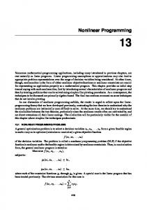
Table 3: The reduction in the number of remaining faults. Examples Initial faults Remaining Reduction (%) faults 1 514.0 172.0 33.6 2 268.7 68.5 25.5 3 276.7 97.4 35.2 3.4.2. Example of minimizing the amount of testing-effort given the number of remaining faults and reliability requirements. Suppose the total number of remaining faults Z is given. We have to allocate the expenditures to each module to minimize the total amount of testing-effort expenditures. Using Algorithm 2 in Section 2.2 and Table 1, the optimal solutions are derived and shown in Table 4. Furthermore, the relationship between the total amount of testing-effort expenditures and the reduction rate of the remaining faults are also depicted in Figure 1.
Table 4: The optimal testing-effort expenditures using algorithm 2. Module X + C* X i + C i* X + C* i
1 2 3 4 5 6 7 8 9 10
i
for ex.1 7700 5013 5643 5424 10211 1770 20220 20131 7759 2388
i
for ex.2 6962 2608 3302 3109 6258 0 2847 5263 0 0
i
for ex.3 5941 2772 3974 4268 8908 0 7931 8919 5595 0
Ci = max{0, D1 , D2 , D3 ,....., D N } Based on the above scenario, if we know how to adjust the consumption rate of testing effort expenditures in the logistic testing effort function (i.e., α2i) at T2, then the project manager can increase the testing-resource expenditures in (T1 , T2 ] . First, from Eq. (2), we know that testing-effort consumption function at T1 for each module is as follows: 1+κ − α κt −( ) N A α κe 1i α κ t − κ 1i 1i 1i 1 i w1iκ (t ) = × 1+ A e 1i κ (43) Therefore, the mean testing-effort consumption function in (T1 , T2 ] is 1+κ − α κt N A α κe 2 i − α κt − ( κ ) w2iκ (t ) = 2i 2i 2i × 1 + A e 2i 2i κ (44) and
( )=
N 2i t
N A α e
− α κt 1i
1i 1i 1i
A α e
− α κt
2i 2i
2i
1 + A1i e 1i × 1 + A e − α 2iκt 2i − α κt
−(
1+κ
κ
)
(45)
where T2 ≥ t > T1 . Applying Eq. (45), we know
Figure 1: The reduction rate of remaining faults vs. the total testing-effort expenditures.
3.5. Testing- resources control problem In order to reduce the risk and achieve a given operational quality at a specified time, we can use SRMGs to estimate and control the required testing effort. The main problem is how to estimate the number of extra faults during module testing which have to be found [6, 17, 22]. Let us consider the following scenario: (1). Due to economic considerations, software testing and debugging will eventually have to stop at a time point, T2. (2). Based on the SRGM selected by the software developers or test teams, for each module its behavior of consuming testing resources during testing is estimated at time T1 (0 0 then
S
5. Conclusions
This research was supported by the National Science Council, Taiwan, ROC., under Grant NSC 90-2213-E-002113 and also substantially supported by a grant from the Research Grant Council of the Hong Kong Special Administrative Region (Project No. CUHK4222/01E). Further, we thank the anonymous referees for their critical review and comments.
7. References S
k
< W − ∑ C k − ξ then i =1
select λ l+1 < λ l Else select λ l+1 > λ l End-if. Step 6: Go to Step 2.
[1]
M. R. Lyu (1996). Handbook of Software Reliability Engineering. McGraw Hill.
[2]
O. Berman and N. Ashrafi, “ Optimization Models for Reliability of Modular Software Systems,”IEEE Trans. on Software Engineering, vol. 19, no. 11, pp. 1119-1123, Nov. 1993.
[3]
D. W. Coit, “Economic Allocation of Test Times for Subsystem-Level Reliability Growth Testing,” IIE Transactions, vol. 30, no. 12, pp. 1143–1151, Dec.1998.
[4]
P. Kubat and H. S. Koch, “Managing Test-Procedure to Achieve Reliable Software,” IEEE Trans. on Reliability, vol. 32, No. 3, pp. 299-303, 1983.
[5]
P. Kubat, “Assessing reliability of Modular Software,” Operation Research Letters, vol. 8, No. 1, pp. 35-41, 1989.
[6]
H. Ohtera and S. Yamada, “Optimal Allocation and Control Problems for Software-Testing Resources,” IEEE Trans. on Reliability, vol. 39, No. 2, pp. 171-176, 1990.
Note that if ri (α ik )(C k + X k )