Benchmarking a MOS-based Algorithm on the BBOB-2010 Noiseless Function Testbed Antonio LaTorre
Santiago Muelas
José M. Peña
Department of Computer Systems Architecture and Technology Facultad de Informática Universidad Politécnica de Madrid, Spain
Department of Computer Systems Architecture and Technology Facultad de Informática Universidad Politécnica de Madrid, Spain
Department of Computer Systems Architecture and Technology Facultad de Informática Universidad Politécnica de Madrid, Spain
[email protected]
[email protected]
[email protected]
ABSTRACT In this contribution, a hybrid algorithm combining Differential Evolution and IPOP-CMA-ES is presented and benchmarked on the BBOB 2010 noiseless testbed. The hybrid algorithm has been constructed within the Múltiple Offspring Sampling framework, which allows the seamless combination of múltiple metaheuristics in a dynamic algorithm capable of adjusting the participation of each of the composing algoritmias according to their current performance. The experimental results show a robust behavior of the algorithm and a good scalability as the dimensionality increases.
Categories and Subject Descriptors G.1.6 [Numerical Analysis]: Optimization—global optimization, unconstrained optimization; F.2.1 [Analysis of Algorithms and Problem Complexity]: Numerical Algorithms and Problems
General Terms Algorithms
Keywords Benchmarking of algorithms, Black-box optimization, Continuous optimization, IPOP-CMA-ES, Differential Evolution, Múltiple Offspring Sampling
1.
INTRODUCTION
In this contribution, a hybrid algorithm constructed by means of the Múltiple Offspring Sampling (MOS) framework has been applied to the Black Box Optimization 2010 Noiseless Function Testbed. This framework allows the combination of different evolutionary models following an HRH (High-level Relay Hybrid) approach (according to Talbi's
taxonomy, briefly reviewed in Section 2) in which the number of evaluations that each algorithm can carry out is dynamically adjusted. For this paper, the IPOP-CMAE-ES [1] and the Differential Evolution (DE) algorithm [8] have been combined within this framework in a multistart strategy and has been benchmarked on 24 different functions. Detailed results regarding the number of evaluations needed to reach a target function on each dimensión along with the CPU times are also given.
2.
ALGORITHM PRESENTATION
Múltiple Offspring Sampling (MOS) is a framework for the development of Dynamic Hybrid Evolutionary Algorithms [6]. MOS provides the functional formalization necessary to design this type of algorithms, as well as the tools to identify and select the best performing configuration for the problem under study. In this context, the hybridization of several algorithms can lead to the following two situations: • A collaborative synergy emerges among the different algorithms that improves the performance of the best one when it is used individually. • A competitive selection of the best one takes place, in which a similar performance (often the same) is obtained with a minimum overhead. In MOS, a key term is the concept of technique, which is a mechanism, decoupled from the main algorithm, to genérate new candidate solutions. This means that, within a MOSbased algorithm, several reproductive mechanisms can be used simultaneously, and it is the main algorithm which selects among the available optimization techniques the most appropriate for the particular problem and search phase. A more concrete definition for these reproductive mechanisms follows: Definition 1. A MOS reproductive technique is a mechanism to créate new individuáis in which: (a) a particular evolutionary algorithm model, (b) an appropriate solution encoding, (c) specific operators (if required), and (d) necessary parameters have been defined. Furthermore, the use of múltiple reproductive mechanisms simultaneously has to be controlled in some way. The MOS framework offers two groups of functions to deal with this
issue: Quality and Participation functions. The first group of functions evalúate how good a set of new individuáis is from the point of view of a desirable characteristic. The second group of functions consider the quality valúes computed by the first group and adjust the number of new individuáis that each reproductive technique will be allowed to genérate in the next step of the search. This way, the algorithm is able to dynamically adjust the participation of each of the available techniques and exploit the benefits of each of them at different stages of the search process. Finally, the Múltiple Offspring Sampling framework allows the development of both HTH (High-level Teamwork Hybrid) and HRH (High-level Relay Hybrid) algorithms (according to Talbi's nomenclature [9]). In the case of the HTH algorithms, two metaheuristics are executed in parallel, working at the same time on the resolution of the problem. On the other hand, in the case of the HRH algorithms, two metaheuristics are executed in sequence, one after the other, and changes of the executing algorithm are carried out according to a given policy. As the proposed algorithm is of the HRH type, more attention will be paid to this type of algorithms. In terms of the MOS framework, the available techniques in a MOS-based HRH hybrid algorithm are used in sequence, one after the other, each of them reusing the output population of the previous technique. This approach fits better when there are non-population-based techniques, such as local searches, as techniques are not constrained to produce a % of the common population. If different population sizes are used by different techniques, it is the responsibility of the technique to make grow/shrink the population in order to adjust it to its needs and to return a population of an appropriate size to the next technique. For example, if a population-based algorithm is combined with a local search, the latter could select one or more individuáis from the output population of the population-based algorithm, modify them as needed and then include them in the original population by means of a predefined elitism procedure. In this type of algorithms, the search process is divided into a fixed number of steps that is established at the beginning of the execution. Each step is assigned an amount of Fitness Evaluations (FESÍ in Algorithm 1), which are distributed by the Participation Function (PF). Each technique can manage its number of allocated FEs at each step of the algorithm (FESi ) in its own particular way. For example, a population-based technique, such as Differential Evolution, could execute several iterations of the algorithm, whereas a Local Search could decide to spend all its assigned evaluations in improving just one individual. The quality of the new individuáis of each technique will be averaged at the end of the whole set of evaluations, as the división of the search into generations depends on each of the techniques. A pseudocode of this approach is given in Algorithm 1. Further information about the MOS framework can be found in [6]. In this contribution, an HRH Dynamic algorithm is proposed. This algorithm combines the explorative/exploitative strength of two heuristic search methods, that separately have proven to obtain very competitive results in either low or high dimensional problems. These algorithms are: the IPOP-CMA-ES algorithm [1], the best algorithm of the '"Specicd Session on Real-Parameter Optimization" held at the CEC 2005 Congress, and the DE algorithm [8] which has demonstrated to obtain competitive results when executed
Algorithm 1 HRH MOS Algorithm 1: Créate initial overall population of candidate solutions Po 2: Uniformly distribute participation among the n used techniques —> Vj lio = ~¡T- Each technique produces a subset of individuáis according to its participation (n o J ) 3: Evalúate initial population Po 4: while number of steps not exceeded do 5: Update Quality of T¡ computed as the average quality of all the individuáis created by technique T¡ in the previous step 6: Update participation ratios from Quality valúes computed in Step 5 - • Vj I T ^ = PF(Q¡j)) 7: Update FEs allocated for each technique at this step: - • Vj FEs¡j)
= n ^
• FESÍ
8: for every available technique Tj do 9: while FEs¿ not exceeded do 10: Evolve 11: end while 12: end for 13: end while
independently and when combined with other algorithms [3, 7]For the adjustment of the participation of each technique in the overall search process, a new Quality Function (QF) has been proposed. This QF takes into account two desirable characteristics in a search algorithm: the Average Fitness Increment of the newly created individuáis after a set of allocated Fitness Evaluations and the number of times that these improvements take place (Equation 1).
QÍ]) = l I T^_1 Ql
^¡-i>^-\
Vj,fce[l,n]
otherwíse
= Quality of technique T¡ in step i
Yyf = Average Fitness Increment of T¡ in step i r¿
= Number of Fitness improvements of T¡ in step i (1) This Quality Function uses the Average Fitness Increment as the effective QF only if there is consensus among both measures. If this is not the case, the raw number of fitness improvements is used. The logic behind this function is that, in some functions, the use of the Average Fitness Increment QF could be very elitist. In some particular situations, a technique which is not carrying out an effective search could introduce, for some reason, a large increment in the average fitness valué of the new individuáis. This could be due, for example, to a recombination of poor solutions. In such a case, it is easy for a technique to improve previous solutions. However, it could be more adequate to carry out small changes to good individuáis in order to find the right "path" to the global optimum rather than carrying out substantial modifications to poor solutions. For this reason, a consensus of both measures is required in order to apply the more elitist Average Fitness Increment QF. If this is not the case, the number of fitness improvements is used to guarantee a softer adjustment of participation.
The quality valúes computed by this QF are used by a Dynamic Participation Function to adjust the number of Fitness Evaluations allocated for each technique at each step (Equation 2). This P F computes, at each step, a trade-off factor for each technique, A¿ , that represents the decrease in participation for the j — th technique at the i — th step, for every technique except the best performing ones. These techniques will increase their participation by the sum of all those A¿ divided by the number of techniques with the best quality valúes.
PFdynW)
=
n ^ + 77
n
(i)
A,-
2-^kébest A r¡ = 1|6esí|
if j e best, otherwise
(2)
(fe)
best = {l / Q¡1) > Q¡m) V í . m e [l,n]} The above-mentioned A¿ valúes are computed as shown in Equation 3. These A¿ factors are computed from the relative difference between the quality of the best and the j — th techniques, n being the number of available techniques. In this equation, £ represents a reduction factor, i.e., the ratio that is transferred from one technique to the other(s) (usually set to a valué of 0.05). Finally, a minimum participation ratio can be established to guarantee that all the techniques are represented through all the search. This is done to avoid, if possible, premature convergence to undesired solutions caused by a technique that obtains all the participation in the early steps of the search and quickly converges to poor regions of the solution space, preventing the other techniques to collaborate at later stages of the process, in which they could be more beneficial. ^(best)
A (i)
-^(best)
M)
TU) nr-i
V j G [ l , n ] / 3 ¿best
3.
Table 1: Computer Configuration PC Intel Xeon 8 cores 1.86Ghz CPU Operating System Ubuntu Linux 8.04 Prog. Language C++ Compiler GNU C + + 4.3.2
Regarding the parameter tuning, no thorough parameter study has been conducted for this work. The parameters of the algorithm were selected based on the extensive parameter tuning that was carried out for the HRH algorithm presented in [7] on a different testbed of functions, and for a similar study that considers the same benchmark of ISDA 2009 and experiments with a MOS based algorithm, submitted for publication to an international journal and currently 1 under review. Table 2 displays the final valúes that were selected for this experimentation, both for the DE, the IPOPCMA-ES and also for the main algorithm. The parameters of the algorithms remain the same for all the functions and, thus, the Crafting Effort (CrE) valué is zero. Table 2: Parameters of the algorithm Parameter Valué Initial Population Size 15 Máximum Pop. Size (after restarts) 6400 DE CR 0.5 DEF 0.5 DE Crossover Operator Exponential DE Selection Operator Tournament 2 DE Model classic Minimum Participation Ratio 5% Number of Steps 85
(3)
To summarize, the presented algorithm works as follows. All the available techniques are allocated the same number of FEs at the beginning of the execution. At the end of each step, the quality of the new solutions created by each technique is evaluated and, based on this quality, its participation ratio is adjusted accordingly. This participation ratio is used to compute the number of FEs that each technique will be allowed to use in the next step of the search. If a minimum participation ratio has been established, then the number of FEs can not go below this threshold. Finally, a restart mechanism, similar to the one used by the IPOP-CMA-ES algorithm, was also used within the proposed algorithm. With this strategy, the algorithm is halted whenever a restart stopping criteria is met, reinitializing the population and increasing its size by a factor of two until a máximum population size is reached. As this restart mechanism depends on some specific conditions of the IPOP-CMAES technique, the restart can only take place when this technique is being executed. However, the effect of the restart affects to all the available techniques, as it is the overall population which is restarted. Moreover, the framework easily allows the use of additional restart mechanisms associated to the remaining techniques or overall restart mechanisms independent of these techniques.
EXPERIMENTAL PROCEDURE
The results reported for this work have been obtained from 15 independent executions executed on the computer configuration displayed in Table 1.
4.
CPU TIMING EXPERIMENT
For the timing experiment the proposed algorithm was run on /g for at least 30 seconds. This experimentation has been conducted on the aforementioned computer configuration depicted in Table 1. The results of this study are reported in Table 3. Table 3: C P U Timing D 2 3 5 10 runs 182 161 143 112 seconds x 10~ 6 3.5 3.9 4.5 4.5
20 82 4.7
40 52 5.8
The CPU-time per function evaluation grows linearly up to 5 dimensions, probably due to the overhead of the hybridization procedures, and then it gets stabilized for dimensions 5, 10 and 20. Finally, for 40 dimensions, the CPU-time starts to grow again, this time due to the increased complexity for this problem size. x
March 2010
20-D
5-D Table 5: ERT loss ratio (see Figure 3) compared to the respective best result from B B O B - 2 0 0 9 for budgets given in the flrst column. The last row R L u s / D gives t h e number of function evaluations in unsuccessful runs divided by dimensión. Shown are t h e smallest, 10%-ile, 25%-ile, 50%-ile, 75%-ile and 90%ile valué (smaller valúes are better). / 1 - / 2 4 in 5-D, maxFE/D=727186 10% 25% med 75% 90% # F E s / D best 2 1.3 1.6 1.9 2.9 4.2 8.5 10 2.3 3.3 3.8 5.1 6.8 50 100 2.8 6.6 8.7 12 16 42 le3 2.2 2.2 3.2 9.3 25 51 le4 0.72 1.6 3.1 6.6 34 1.3e2 le5 1.2 1.6 3.1 5.6 17 2.5e2 le6 0.52 1.2 2.6 4.7 16 2.7e2 RLus/D le5 le5 le5 le5 2e5 3e5 / l - / 2 4 in 20-D, maxFE/D=199139 #FEs/D Dest 10% 25% med 75% 90% 2 1.0 2.4 9.4 31 40 40 10 4.8 6.9 10 51 2.0e2 2.0e2 100 5.6 6.5 8.8 17 24 47 le3 0.26 1.6 3.2 9.8 44 1.4e2 le4 0.09 1.1 2.0 3.9 67 2.8e2 le5 0.07 0.94 2.1 4.0 14 2.2e2 le6 0.07 0.94 2.1 4.4 30 1.3e2 RLus/D le5 le5 le5 le5 2e5 2e5
• !
"•"
1
"*•
1
•
:
fl-5
V 1 0
^
t^ ^-
t
+
+
í
+
+ -i-
1
-•>
re-9 3 2
*—É-
o
t^-t
1
4
+ -F =t ^ " f - ^ -u 4+ ;F
1
2
#
4
%
3 fl0-14
+ + 1
5.
• !
^L — r^
t * ^ í ^
RESULTS
Results from experiments according to [4] on the benchmark functions given in [2, 5] are presented in Figures 1, 2 and 3 and in Tables 4 and 5. The overall results in the noiseless testbed are quite satisfactory in terms of achieved precisión and scalability. The hybrid algorithm here presented is able to sol ve 24, 24, 24, 24, 21 and 20 functions out of 24 in 2, 3, 5, 10, 20 and 40 dimensions, respectively. Compared to the individual use of its composing algorithms, the hybrid algorithm obtains more stable results than any of them. Furthermore, functions / 3 and / 4 which are practically unsolvable for the IPOP-CMA-ES algorithm, are now solved thanks to the hybridization with the DE algorithm. On the other hand, the most difñcult function for our approach is /24, for which convergence is never reached for dimensión 20 or above. Nevertheless, this is somehow reasonable, as this function has been designed to be deceptive for Evolution Strategies (and the DE is also unable to deal with it). Furthermore, it can also be observed that the proposed algorithm achieves one of the best results in terms of ECDFs valúes, compared with the algorithms presented in the previous BBOB-2009 workshop, for all the groups of functions, as it can be seen in Figure 2. Finally, regarding the number of Fitness Evaluations required to reach a particular precisión, it can be higher than for other algorithms, such as the IPOP-CMA-ES when it is used individually. This is normal, as the regulatory mechanisms implemented by the MOS framework need some time to take a decission and adjust the participation of each technique accordingly.
fl5-l4
+
t
i
+ ^-f—-L i
!
:
:
i i
i
* + í^^~~f
;
-
+ ^
+
w* 1 2 3 4 loglO of FEvals / dimensión
± *
1 2 3 4 loglO of FEvals / dimensión
Figure 3: ERT loss ratio versus given budget FEvals. The target valué ft for ERT (see Figure 1) is t h e smallest (best) recorded function valué such that ERT(/ t ) < FEvals for the presented algorithm. Shown is FEvals divided by the respective best ERT(/t) from B B O B - 2 0 0 9 for functions /1-/24 in 5-D and 2 0 - D . Each ERT is multiplied by exp(CrE) correcting for the parameter crafting effort. Line: geometric mean. Box-Whisker error bar: 25-75%-ile with median (box), 10-90%-ile (caps), and mínimum and máximum ERT loss ratio (points). The vertical line gives the maximal number of function evaluations in this function subset.
1 5p
!
!—!
m 0-+"':::::i
2
2 Ellipsoid separable
Sphere
1 1i
v
— -
-
5 10 20 5 Linear slope
+1 i +0 -1 i -2 -3 -5 -8
40
M* * 2
3
5
10
20
40
2
3
6 Attractlve sector 4-4
í
* •
* *
4 Slcew Rastrlgln-Bueche separable =—] M
14
i i
3
3 Rastrigin separable
i
9
#
5 10 20 7 Step-ellipsoid
^
4
tfU
Jd i
2
3
5 10 20 8 Rosenbrock original
40
*| t •
o M 2
3
.
5
5 10 20 9 Rosenbrock rotated
10 10 Ellipsoid
2
20
10
20
4C
2
'••-''-•M
\ + 4
g*
2 1
ni
0
o[
5
c
20
40
* i 11
1% ^ ¥
14 Sum of different powers
10
iíáí»*
5
¥^
5
12 Bentcigar
4 3
13 Sharp ridge
3
11 Discus
*
i
¡
10 15 Rastrigin
20
2
3
¥
*
*
5 10 20 16 Weierstrass
"41 8
V * • 2 17 Schaffer F7, condition 10
3 5 10 20 40 18 Schaffer F7, condition 1000
3 5 10 20 40 19 Griewank-Rosenbrock F8F2
5 10 20 20 Schwefel x*sin(x)
40
Ü=P • ¿ : 2
3
5
10
•
+
:
20
40
*
\
*
•
•
•
23 Katsuuras
ottss; 2
3
5 10 20 24 Lunacek bi-Rastrigin
^ 40
* *
f * • 2
3
5
10
20
40
Figure 1: Expected Running Time (ERT, • ) to reach / op t + A / and median number of /-evaluations from successful triáis (+), for A / = Í O " ^ 1 ' 0 ' - 1 ' - 2 ' - 3 ' - 5 ' - 8 ' (the exponent is given in the legend of /i and /24) versus dimensión in log-log presentation. For each function and dimensión, ERT(A/) equals to #FEs(A/) divided by the number of successful triáis, where a trial is successful if / op t + A / was surpassed. The #FEs(A/) are the total number (sum) of /-evaluations while / op t + A / was not surpassed in the trial, from all (successful and unsuccessful) triáis, and / op t is the optimal function valué. Crosses (x) indícate the total number of /-evaluations, #FEs(—oo), divided by the number of triáis. Numbers above ERT-symbols indícate the number of successful triáis. Y-axis annotations are decimal logarithms. The thick light line with diamonds shows the single best results from BBOB-2009 for A / = 1CP8. Additional grid lines show linear and quadratic scaling.
/ l in 5-D, N = 1 5 , m F E = 3 1 4 4 / l in 2 0 - D , N = 1 5 , m F E = 1 0 1 0 1 # ERT 10% 90% R T S U C c: # ERT 10% 90% RTSUCC 15 7 . l e í 2 . 0 e 0 1 . 3 e 2 7.leí 15 1 . 5 e 3 1 . 3 e 3 2 . 0 e 3 1.5e3 15 4 . 0 e 2 2 . 3 e 2 5 . 5 e 2 4.0e2 15 2 . 5 e 3 2 . 4 e 3 2 . 6 e 3 2.5e3 15 8 . 1 e 2 7 . 2 e 2 9 . 2 e 2 8.1e2 15 2 . 9 e 3 2 . 9 e 3 3 . 0 e 3 2.9e3 15 1 . 5 e 3 1 . 4 e 3 1 . 6 e 3 1.5e3 15 5 . 3 e 3 5 . 1 e 3 5 . 5 e 3 5.3e3 15 2 . 1 e 3 1 . 8 e 3 2 . 3 e 3 2.1e3 15 6 . 4 e 3 5 . 9 e 3 7 . 0 e 3 6.4e3 15 3 . 0 e 3 2 . 9 e 3 3 . 1 e 3 3.0e3 15 9 . 1 e 3 8 . 8 e 3 1.0 e 4 9.1e3 fS ¡ n 5 - D , N = 1 5 , m F E = 2 0 4 2 3 / 3 in 2 0 - D , N = 15, m F E = 1 8 4 1 6 0 # ERT 10% 90% RTSUCC # ERT 10% 90% RTSUCC A/ 10 15 l . l e 3 8 . 8 e 2 1 . 6 e 3 1.1 e 3 15 2 . 4 e 4 9 . 4 e 3 5 . 1 e 4 2.4e4 1 15 2 . 7 e 3 2 . 4 e 3 3 . 4 e 3 2.7e3 15 5 . 6 e 4 1 . 5 e 4 1.2 e 5 5.6e4 l e - 1 15 4 . 0 e 3 2 . 6 e 3 4 . 1 e 3 4.0e3 15 6 . 8 e 4 1 . 7 e 4 1 . 4 e 5 6.8e4 l e - 3 15 5 . 3 e 3 4 . 0 e 3 5 . 4 e 3 5.3e3 15 7 . 5 e 4 2 . 1 e 4 1.5 e 5 7.5e4 l e - 5 15 6 . 2 e 3 4 . 9 e 3 6 . 2 e 3 6.2e3 15 8 . 2 e 4 2 . 5 e 4 1.6 e 5 8.2e4 l e - 8 15 7 . 7 e 3 6 . 4 e 3 7 . 6 e 3 7.7e3 15 9 . 5 e 4 3 . 1 e 4 1 . 7 e 5 9.5e4 / 5 ¡n 5 - D , N = 1 5 , m F E = 650 / 5 ¡n 2 0 - D , N = 1 5 , m F E = 2200 # ERT 10% 90% RTSUCc # ERT 10% 90% RTSUCC A/ 10 15 2 . 0 e 2 8 . S e l 2 . 9 e 2 2.0eS 15 2 . 1 e 3 2 . 0 e 3 2 . 2 e 3 2.1e3 1 15 4 . 2 e 2 3 . 0 e 2 5 . 8 e 2 4.2eS 15 2 . 1 e 3 2 . 1 e 3 2 . 2 e 3 2.1e3 l e - 1 15 5 . 0 e 2 3 . 3 e 2 6 . 3 e 2 5.0eS 15 2 . 1 e 3 2 . 1 e 3 2 . 2 e 3 2.1e3 l e - 3 15 5 . 1 e 2 3 . 3 e 2 6 . 3 e 2 5.1eS 15 2 . 1 e 3 2 . 1 e 3 2 . 2 e 3 2.1e3 l e - 5 15 5 . 1 e 2 3 . 3 e 2 6 . 3 e 2 5.1eS 15 2 . 1 e 3 2 . 1 e 3 2 . 2 e 3 2.1e3 l e - 8 15 5 . 1 e 2 3 . 3 e 2 6 . 3 e 2 5.1eS 15 2 . 1 e 3 2 . 1 e 3 2 . 2 e 3 2.1e3 f7 i n 5 - D , N = 1 5 , m F E = 6 8 8 7 f7 ¡ n 2 0 - D , N = 1 5 , m F E = 5 3 3 5 7 # E R T 1 0 % 9 0 % R T # E R T 1 0 % 9 0 % R TSUCC A/ SUCC 10 15 3 . 0 e 2 1 . 5 e 2 6 . 1 e 2 3.0e2 15 3 . 6 e 3 2 . 8 e 3 5 . 0 e 3 3.6e3 1 15 1 . 6 e 3 7 . 6 e 2 3 . 9 e 3 1.6e3 15 2 . 6 e 4 1 . 5 e 4 3 . 9 e 4 2.6e4 l e - 1 15 2 . 9 e 3 1 . 4 e 3 5 . 2 e 3 2.9e3 15 3 . 7 e 4 2 . 1 e 4 4 . 6 e 4 3.7e4 l e - 3 15 3 . 6 e 3 2 . 1 e 3 6 . 0 e 3 3.6e3 15 3 . 9 e 4 2 . 3 e 4 4 . 8 e 4 3.9e4 l e - 5 15 3 . 6 e 3 2 . 1 e 3 6 . 0 e 3 3.6e3 15 3 . 9 e 4 2 . 3 e 4 4 . 8 e 4 3.9e4 l e - 8 15 3 . 8 e 3 2 . 1 e 3 6 . 5 e 3 3.8e3 15 4 . 0 e 4 2 . 4 e 4 4 . 8 e 4 4.0e4 / 9 ¡n 5 - D , N = 1 5 , m F E = 1 7 8 8 3 / 9 ¡n 2 0 - D , N = 1 5 , m F E = 249530 # ERT 10% 90% RTSUCC # ERT 10% 90% RTSUCC A/ 10 15 4 . 5 e 2 4 . 1 e 2 4 . 8 e 2 4.5e2 15 1 . 6 e 4 1.1 e 4 2 . 1 e 4 1.6e4 1 15 1 . 3 e 3 7 . 6 e 2 1.6 e 3 1.3e3 15 3 . 6 e 4 2 . 7 e 4 4 . 2 e 4 3.6e4 l e - 1 15 3 . 6 e 3 2 . 1 e 3 8 . 0 e 3 3.6e3 15 4 . 8 e 4 3 . 1 e 4 4 . 6 e 4 4.8e4 l e - 3 15 5 . 2 e 3 3 . 1 e 3 1 . 4 e 4 5.2e3 15 5 . 3 e 4 3 . 4 e 4 4 . 9 e 4 5.3e4 l e - 5 15 5 . 7 e 3 3 . 7 e 3 1.5 e 4 5.7e3 15 5 . 4 e 4 3 . 6 e 4 5 . 0 e 4 5.4e4 l e - 8 15 6 . 4 e 3 4 . 4 e 3 1.5 e 4 6.4e3 15 5 . 6 e 4 3 . 8 e 4 5 . 2 e 4 5.6e4 / l l in 5 - D , N = 1 5 , m F E = 5992 / l l in 2 0 - D , N = 15, m F E = 38386 # ERT 10% 90% RTSUCC # ERT 10% 90% RTSUCC A/ 10 15 2 . 5 e 3 1 . 7 e 3 2 . 9 e 3 2.5e3 15 2 . 1 e 4 1 . 8 e 4 2 . 6 e 4 2 .1 e 4 1 15 3 . 3 e 3 3 . 0 e 3 3 . 7 e 3 3.3e3 15 2 . 3 e 4 2 . 0 e 4 2 . 7 e 4 2.3e4 l e - 1 15 3 . 8 e 3 3 . 6 e 3 4 . 2 e 3 3.8e3 15 2 . 5 e 4 2 . 3 e 4 2 . 9 e 4 2.5e4 l e - 3 15 4 . 4 e 3 4 . 2 e 3 4 . 5 e 3 4.4e3 15 2 . 8 e 4 2 . 6 e 4 3 . 2 e 4 2.8e4 l e - 5 15 4 . 8 e 3 4 . 5 e 3 5 . 2 e 3 4.8e3 15 3 . 0 e 4 2 . 7 e 4 3 . 5 e 4 3.0e4 l e - 8 15 5 . 6 e 3 5 . 2 e 3 5 . 9 e 3 5.6e3 15 3 . 3 e 4 3 . 0 e 4 3 . 7 e 4 3.3e4 / l 3 ¡n 5 - D , N = 15, m F E = 8 3 8 9 / 1 3 in 2 0 - D , N = 1 5 , m F E = 1 5 4 0 4 0 # ERT 10% 90% RTSUCC # ERT 10% 90% RTSUCC A/ 10 15 1 . 4 e 3 1 . 2 e 3 1 . 7 e 3 1.4e3 15 6 . 4 e 3 5 . 2 e 3 5 . 9 e 3 6.4e3 1 15 2 . 3 e 3 2 . 1 e 3 2 . 8 e 3 2.3e3 15 1 . 8 e 4 7 . 8 e 3 3 . 2 e 4 1.8e4 l e - 1 15 3 . 4 e 3 2 . 9 e 3 3 . 8 e 3 3.4e3 15 3 . 2 e 4 8 . 9 e 3 5 . 3 e 4 3.2e4 l e - 3 15 4 . 6 e 3 4 . 2 e 3 5 . 1 e 3 4.6e3 15 5 . 2 e 4 2 . 8 e 4 8 . 5 e 4 5.2e4 l e - 5 15 5 . 9 e 3 5 . 3 e 3 6 . 6 e 3 5.9e3 15 7 . 8 e 4 6 . 3 e 4 1.0 e 5 7.8e4 l e - 8 15 7 . 7 e 3 7 . 3 e 3 8 . 2 e 3 7.7e3 15 1 . 0 e 5 6 . 9 e 4 1.5 e 5 1.0e5 / 1 5 ¡n 5 - D , N = 1 5 , m F E = 75737 / 1 5 in 2 0 - D , N = 1 5 , m F E = 5 4 5 9 8 7 # ERT 10% 90% RTSUCC # ERT 10% 90% RTSUCC A/ 10 15 2 . 2 e 3 l . l e 3 3 . 0 e 3 2.2e3 L5 4 . 6 e 4 3 . 9 e 4 7 . 5 e 4 4.6 e4 1 15 1 . 3 e 4 3 . 1 e 3 2 . 3 e 4 1.3e4 L5 2 . 3 e 5 1 . 6 e 5 3 . 0 e 5 2.3e5 l e - 1 15 3 . 1 e 4 1 . 3 e 4 6 . 4 e 4 3.1 e4 L5 3 . 1 e 5 1 . 6 e 5 4 . 7 e 5 3.1e5 l e - 3 15 3 . 3 e 4 1 . 4 e 4 6 . 6 e 4 3.3e4 L5 3 . 2 e 5 1 . 7 e 5 4 . 8 e 5 3.2e5 l e - 5 15 3 . 4 e 4 1 . 5 e 4 6 . 7 e 4 3.4e4 L5 3 . 3 e 5 1 . 8 e 5 5 . 0 e 5 3.3e5 l e - 8 15 3 . 5 e 4 1 . 6 e 4 7 . 1 e 4 3.5e4 L5 3 . 4 e 5 1 . 9 e 5 5 . 2 e 5 3.4e5 / 1 7 in 5-D, N = 1 5 , m F E = 1 8 9 7 8 4 / 1 7 in 2 0 - D , N = 1 5 , m F E = 1 9 7 5 9 4 # ERT 10% 90% RTSUCC # ERT 10% 90% RTSUCC A/ 10 15 1 . 4 e l 2 . 0 e 0 3 . 6 e l 1.4el 15 6 . 9 e 2 2 . 5 e 2 1.0 e 3 6.9e2 1 15 1 . 3 e 3 8 . 0 e 2 2 . 7 e 3 1.3e3 15 8 . 5 e 3 2 . 7 e 3 6 . 3 e 3 8.5e3 l e - 1 15 4 . 7 e 3 1 . 6 e 3 1.6 e 4 4.7e3 15 1.1 e 4 5 . 5 e 3 9 . 0 e 3 1.1 e 4 l e - 3 15 2 . 0 e 4 3 . 1 e 3 6 . 7 e 4 2.0e4 15 3 . 5 e 4 1.1 e 4 4 . 5 e 4 3.5e4 l e - 5 15 2 . 5 e 4 4 . 5 e 3 9 . 7 e 4 2.5e4 15 6 . 8 e 4 4 . 7 e 4 9 . 7 e 4 6.8e4 l e - 8 15 3 . 2 e 4 6 . 8 e 3 1.0 e 5 3.2e4 15 1 . 0 e 5 5 . 7 e 4 1.1 e 5 1.0e5 / 1 9 ¡n 5 - D , N = 15, m F E = 564073 / 1 9 in 2 0 - D , N = 15, m F E = 2.28e6 # E R T 1 0 % 9 0 % R T # E R T 1 0 % 9 0 % R T A/ SUCC SUCC 10 15 2 . 7 e l 1 . 2 e l 5 . 2 e l 2.7el 15 1 . 2 e 3 8 . 8 e 2 1 . 5 e 3 1.2e3 1 15 6 . 6 e 2 4 . 8 e 2 9 . 7 e 2 6.6 e2 15 2 . 1 e 4 9 . 0 e 3 4 . 2 e 4 2.1 e4 l e - 1 15 2 . 6 e 4 2 . 5 e 3 1.1 e 5 2.6 e4 11 1 . 0 e 6 3 . 9 e 4 2 . 5 e 6 2.8e5 le-3 9 5.8e5 4 . 9 e 3 1.4e6 2.3 e5 0 47e-3 84e-4 2Q&-2 2.0e6 le-5 9 5.8e5 5 . 3 e 3 1.4e6 2.3 e5 le-8 9 5.8e5 6 . 4 e 3 1.4e6 2.3 e5 / 2 1 ¡n 5 - D , N = 15, m F E = 3.64e6 / 2 1 ¡n 2 0 - D , N = 1 5 , m F E = 3 . 8 5 e 6 # ERT 10% 90% RTSUCC # ERT 10% 90% RTSUCC A/ 10 15 1.9e2 2 . 3 e l 3 . 8 e 2 1.9e2 15 6 . 0 e 3 2 . 1 e 3 2 .1 e 4 6 . 0 e3 1 15 7.9 e 4 5 . 8 e 2 3 . 8 e 5 7.9e4 11 1 . 7 e 6 2 . 4 e 3 5 . 4 e 6 3.5 e5 l e - 1 15 4 . 7 e 5 7 . 2 e 2 1 . 5 e 6 4.7e5 8 4.0e6 2.7e3 9.8e6 7.6e5 l e - 3 13 8 . 3 e 5 1 . 3 e 3 3 . 6 e 6 2.7e5 8 4 . 0 e 6 4 . 2 e 3 1.1 e 7 7.7e5 l e - 5 13 8 . 4 e 5 1 . 5 e 3 3 . 6 e 6 2.8e5 8 4 . 0 e 6 5 . 4 e 3 1.1 e 7 7.9e5 l e - 8 13 9 . 9 e 5 2 . 1 e 3 3 . 6 e 6 4.4e5 8 4 . 1 e 6 7 . 5 e 3 1.1 e 7 8.1e5 / 2 3 ¡n 5 - D , N = 1 5 , m F E = 5 8 4 8 9 6 / 2 3 ¡n 2 0 - D , N = 1 5 , m F E = 2 . 1 1 e 6 # ERT 10% 90% RTSUCC # ERT 10% 90% RTSUCC A/ 10 15 6 . 7 e 0 2 . 0 e 0 1 . 4 e l 6.7e0 15 6 . 9 e 0 l . O e O 1 . 5 e l 6 . 9 eO 1 15 8 . 5 e 3 2 . 4 e 3 1.6 e 4 8.5e3 15 9 . 1 e 4 2 . 1 e 4 1 . 9 e 5 9.1 e4 l e - 1 15 5 . 8 e 4 9 . 5 e 3 1.1 e 5 5.8e4 13 6 . 0 e 5 2 . 5 e 4 2 . 0 e 6 2.9 e5 l e - 3 15 1 . 2 e 5 l . l e 4 3 . 1 e 5 1.2e5 0 29e-3 50e-4 25e-2 7.1e5 l e - 5 14 1 . 3 e 5 1 . 2 e 4 3 . 2 e 5 9.0e4 l e - 8 14 1 3 e 5 1 . 3 e 4 3 . 2 e 5 9.3e4 A/ 10 1 le-1 le-3 le-5 le-8
A/ 10 1 le-1 le-3 le-5 le-8 A/ 10 1 le-1 le-3 le-5 le-8 A/ 10 1 le-1 le-3 le-5 le-8 A/ 10 1 le-1 le-3 le-5 le-8 A/ 10 1 le-1 le-3 le-5 le-8 A/ 10 1 le-1 le-3 le-5 le-8 A/ 10 1 le-1 le-3 le-5 le-8 A/ 10 1 le-1 le-3 le-5 le-8 A/ 10 1 le-1 le-3 le-5 le-8 A/ 10 1 le-1 le-3 le-5 le-8 A/ 10 1 le-1 le-3 le-5 le-8 A/ 10 1 le-1 le-3 le-5 le-8
/ 2 ¡n 5 - D , N = 15, m F E = 7050 ti i n 2 0 - D , N = 1 5 , m F E = 4 5 9 4 3 # ERT 10% 90% RTSUCC # ERT 10% 90% RTSUCC 15 1.9e3 1.7e3 2 . 4 e 3 1.9 e 3 15 1 . 7 e 4 1.0 e 4 2 . 9 e 4 1 ,7e4 15 2 . 5 e 3 2 . 4 e 3 3 . 0 e 3 2.5 e3 15 1 . 9 e 4 1 . 3 e 4 3 . 3 e 4 1 ,9e4 15 3 . 1 e 3 2 . 4 e 3 3 . 4 e 3 3.1 e3 15 2 . 2 e 4 1 . 5 e 4 3 . 6 e 4 2 ,2e4 15 4 . 1 e 3 3 . 9 e 3 4 . 7 e 3 4.1e3 15 2 . 6 e 4 1 . 9 e 4 4 . 1 e 4 2 ,6e4 15 5 . 0 e 3 4 . 6 e 3 5 . 6 e 3 5.0 e3 15 2 . 9 e 4 2 . 2 e 4 4 . 2 e 4 2 ,9e4 15 6 . 4 e 3 5 . 5 e 3 6 . 9 e 3 6.4e3 15 3 . 4 e 4 2 . 8 e 4 4 . 4 e 4 3,4e4 / 4 in 5 - D , N = 15, m F E = 22862 / 4 in 2 0 - D , N = 15, m F E = 1 8 4 6 8 7 # ERT 10% 90% RTSUCC # ERT 10% 90% RTSUCC 15 1.3e3 8 . 7 e 2 1 . 7 e 3 1.3 e 3 15 4 . 9 e 4 1 . 4 e 4 6 . 3 e 4 4.9e4 15 5 . 8 e 3 3 . 1 e 3 1 . 4 e 4 5.8e3 15 9 . 4 e 4 5 . 8 e 4 1 . 3 e 5 9.4e4 15 9 . 4 e 3 3 . 4 e 3 1 . 6 e 4 9.4e3 15 1 . 0 e 5 6 . 2 e 4 1 . 4 e 5 1.0 e 5 15 l . l e 4 4 . 8 e 3 1 . 8 e 4 1.1 e 4 15 l . l e 5 6 . 8 e 4 1 . 5 e 5 1.1 e 5 15 1.2e4 6 . 3 e 3 2 . 0 e 4 1.2 e 4 15 1 . 2 e 5 7 . 4 e 4 1 . 6 e 5 1.2e5 15 1.4e4 7 . 7 e 3 2 . 2 e 4 1.4e4 15 1 . 4 e 5 8 . 5 e 4 1.8e5 1.4e5 / 6 ¡n 5 - D , N = 15, m F E = 7366 / 6 ¡n 2 0 - D , N = 15, m F E = 29420 # ERT 10% 90% RTSUCC # ERT 10% 90% RT 15 9 . 1 e 2 5 . 0 e 2 1 . 5 e 3 9.1 e2 15 7 . 2 e 3 5 . 5 e 3 8 . 4 e 3 7 2e3 15 1 . 8 e 3 1 . 5 e 3 2 . 2 e 3 1.8e3 15 9 . 1 e 3 8 . 2 e 3 1.1 e 4 9 le3 15 2 . 5 e 3 2 . 1 e 3 2 . 9 e 3 2.5 e3 15 1.1 e 4 1.1 e 4 1 . 4 e 4 1 le4 15 3 . 7 e 3 3 . 2 e 3 4 . 0 e 3 3.7e3 15 1 . 6 e 4 1 . 5 e 4 1 . 7 e 4 1 6e4 15 4 . 9 e 3 4 . 5 e 3 5 . 3 e 3 4.9e3 15 2 . 0 e 4 1 . 9 e 4 2 . 1 e 4 2 0e4 15 6 . 8 e 3 6 . 2 e 3 7 . 3 e 3 6.8e3 15 2 . 6 e 4 2 . 4 e 4 2 . 7 e 4 2 6e4 / 8 ¡n 5 - D , N = 15, m F E = 7515 / 8 ¡n 2 0 - D , N = 15, m F E = 122595 # ERT 10% 90% RTSUCC # ERT 10% 90% RTSUCC 15 8 . 0 e 2 7 . 0 e 2 1 . 0 e 3 8.0e2 15 2 . 3 e 4 1 . 8 e 4 3 . 0 e 4 2 ,3e4 15 2 . 9 e 3 2 . 1 e 3 3 . 6 e 3 2.9 e3 15 4 . 7 e 4 3 . 3 e 4 8 . 8 e 4 4,7e4 15 4 . 1 e 3 3 . 4 e 3 5 . 0 e 3 4.1e3 15 5 . 1 e 4 3 . 8 e 4 9 . 6 e 4 5,le4 15 5 . 1 e 3 4 . 3 e 3 6 . 0 e 3 5.1 e3 15 5 . 4 e 4 4 . 1 e 4 1 . 0 e 5 5 ,4e4 15 5 . 7 e 3 5 . 0 e 3 6 . 6 e 3 5.7e3 15 5 . 6 e 4 4 . 2 e 4 1.0 e 5 5 ,6e4 15 6 . 4 e 3 5 . 7 e 3 7 . 5 e 3 6.4e3 15 5 . 8 e 4 4 . 4 e 4 l . l e 5 5 ,8e4 / l O ¡n 5 - D , N = 15, m F E = 13486 / 1 0 in 2 0 - D , N = 15, m F E = 4 0 0 1 3 # ERT 10% 90% RTSUCC # ERT 10% 90% RTSUCC 15 3 . 4 e 3 2 . 3 e 3 3 . 6 e 3 3.4e3 15 2 . 5 e 4 2 . 1 e 4 2 . 8 e 4 2.5e4 15 4 . 1 e 3 2 . 9 e 3 4 . 0 e 3 4.1e3 15 2 . 9 e 4 2 . 6 e 4 3 . 2 e 4 2.9e4 15 4 . 4 e 3 3 . 0 e 3 4 . 3 e 3 4.4e3 15 3 . 2 e 4 3 . 1 e 4 3 . 3 e 4 3.2e4 15 4 . 8 e 3 3 . 7 e 3 4 . 6 e 3 4.8e3 15 3 . 5 e 4 3 . 3 e 4 3 . 6 e 4 3.5e4 15 5 . 3 e 3 4 . 4 e 3 5 . 1 e 3 5.3e3 15 3 . 7 e 4 3 . 6 e 4 3 . 8 e 4 3.7e4 15 6 . 0 e 3 5 . 0 e 3 5 . 9 e 3 6.0e3 15 3 . 8 e 4 3 . 8 e 4 3 . 9 e 4 3.8e4 / 1 2 in 5 - D , N = 15, m F E = 20426 / 1 2 in 2 0 - D , N = 1 5 , m F E = 2 1 3 1 6 3 # ERT 10% 90% RTSUCC # ERT 10% 90% RTSUCC 15 2 . 7 e 3 1 . 8 e 3 4 . 2 e 3 2.7e3 15 7 . 4 e 3 6 . 0 e 3 8 . 0 e 3 7.4e3 15 4 . 3 e 3 2 . 2 e 3 8 . 8 e 3 4.3e3 15 1.7e4 7 . 8 e 3 3.0 e 4 1.7e4 15 5 . 8 e 3 2 . 7 e 3 1.2 e 4 5.8e3 15 3 . 7 e 4 8 . 6 e 3 4 . 1 e 4 3.7e4 15 7 . 4 e 3 4 . 5 e 3 1 . 4 e 4 7.4e3 15 5 . 0 e 4 2 . 9 e 4 5 . 2 e 4 5.0e4 15 9 . 0 e 3 5 . 6 e 3 1 . 7 e 4 9.0e3 15 5 . 9 e 4 3 . 7 e 4 6 . 0 e 4 5.9e4 15 1.1 e 4 6 . 2 e 3 1. 9 e 4 1.1 e 4 15 6 . 7 e 4 4 . 5 e 4 6 . 8 e 4 6.7e4 / 1 4 i n 5 - D , N = 15, m F E = 6 5 1 7 / 1 4 in 2 0 - D , N = 1 5 , m F E = 4 4 7 0 0 # ERT 10% 90% RTSUCC # ERT 10% 90% RTSUCC 15 2 . 9 e l l . O e O 6 . 3 e l 2.9el 15 1.5e3 1.0e3 1.8e3 1.5e3 15 5 . 3 e 2 3 . 5 e 2 7 . 6 e 2 5.3 e2 15 2 . 5 e 3 2 . 3 e 3 2 . 6 e 3 2.5e3 15 8 . 4 e 2 5 . 9 e 2 l . l e 3 8.4e2 15 3 . 2 e 3 2 . 9 e 3 3 . 8 e 3 3.2e3 15 1 . 9 e 3 1 . 5 e 3 2 . 3 e 3 1.9 e 3 1 5 1.1 e 4 1.1 e 4 1 . 2 e 4 1.1 e 4 15 3 . 6 e 3 3 . 4 e 3 3 . 9 e 3 3.6 e3 15 2 . 3 e 4 2 . 2 e 4 2 . 4 e 4 2.3e4 15 5 . 8 e 3 5 . 4 e 3 6 . 1 e 3 5.8e3 15 4 . 3 e 4 4 . 1 e 4 4 . 4 e 4 4.3 e4 / l 6 ¡n 5 - D , N = 15, m F E = 1.30e6 / 1 6 in 2 0 - D , N = 1 5 , mF E = 3.01e6 # ERT 10% 90% RTSUCC # ERT 10% 90% RTSUCC 15 2 . 0 e 2 5 . 6 e l 3 . 3 e 2 2.0e2 15 2 . 4 e 3 2 . 0 e 3 2 . 8 e 3 2.4e3 15 1 . 8 e 3 6 . 9 e 2 2 . 2 e 3 1.8e3 15 7 . 3 e 3 5 . 2 e 3 6 . 0 e 3 7.3e3 15 6 . 9 e 3 1 . 2 e 3 1 . 8 e 4 6.9e3 15 3 . 8 e 4 8 . 7 e 3 1.2e5 3.8e4 15 1 . 3 e 4 2 . 1 e 3 2 . 1 e 4 1.3e4 12 1 . 0 e 6 7 . 2 e 4 3 . 2 e 6 3.0e5 15 9 . 0 e 4 2 . 9 e 3 2 . 2 e 4 9.0e4 12 l . l e 6 7 . 5 e 4 3 . 2 e 6 3.9e5 15 9 . 4 e 4 3 . 7 e 3 2 . 3 e 4 9.4e4 11 1 . 4 e 6 8 . 0 e 4 3 . 5 e 6 3.3e5 / l 8 ¡n 5 - D , N = 15, m F E = 77728 / 1 8 in 2 0 - D , N = 1 5 , mF E = 375028 # ERT 10% 90% RTSUCC # ERT 10% 90% RTSUCC 15 5 . 0 e 2 3 . 2 e l 8 . 5 e 2 5.0 e2 15 2 . 5 e 3 2 . 3 e 3 3 . 0 e 3 2.5e3 15 2 . 5 e 3 1 . 4 e 3 5 . 4 e 3 2.5 e3 15 6 . 4 e 3 5 . 1 e 3 1 . 2 e 4 6.4e3 15 1 . 2 e 4 2 . 1 e 3 2 . 5 e 4 1.2 e 4 15 2 . 2 e 4 8 . 0 e 3 5 . 0 e 4 2.2e4 15 1 . 6 e 4 3 . 8 e 3 4 . 1 e 4 1.6 e 4 15 8 . 5 e 4 4 . 7 e 4 1 . 7 e 5 8.5e4 15 1 . 8 e 4 5 . 6 e 3 4 . 5 e 4 1.8e4 15 1 . 6 e 5 9 . 9 e 4 2 . 1 e 5 1.6e5 15 2 . 6 e 4 7 . 5 e 3 5 . 4 e 4 2.6 e4 15 1 . 8 e 5 l . l e 5 2 . 3 e 5 1.8e5 / 2 0 ¡n 5 - D , N = 15, m F E = 279314 / 2 0 ¡ n 2 0 - D , N = 1 5 , ir F E = 9 4 1 1 0 5 # ERT 10% 90% RTSUCC # ERT 10% 90% RTSUCC 15 1 . 6 e 2 5 . 5 e l 2 . 3 e 2 1.6e2 15 1 . 7 e 3 1 . 7 e 3 1.8e3 1.7e3 15 2 . 3 e 3 1 . 6 e 3 3 . 5 e 3 2.3e3 15 4 . 5 e 4 2 . 0 e 4 6 . 1 e 4 4.5e4 15 1 . 6 e 4 4 . 1 e 3 3 . 0 e 4 1.6e4 15 2 . 4 e 5 2 . 2 e 5 2 . 8 e 5 2.4e5 15 3 . 0 e 4 8 . 4 e 3 4 . 9 e 4 3.0e4 15 3 . 2 e 5 2 . 9 e 5 3 . 5 e 5 3.2e5 15 5 . 5 e 4 2 . 4 e 4 1 . 0 e 5 5.5e4 15 3 . 6 e 5 3 . 3 e 5 4 . 0 e 5 3.6e5 15 6 . 5 e 4 2 . 8 e 4 l . l e 5 6.5e4 15 4 . 2 e 5 3 . 5 e 5 4 . 3 e 5 4.2e5 / 2 2 ¡n 5 - D , N = 15, m F E = 2.73e6 / 2 2 ¡n 2 0 - D , N = 1 5 , m F E = 3 . 9 8 e 6 # ERT 10% 90% RTSUCC # ERT 10% 90% RTSUCC 15 2 . 6 e 2 5 . 7 e l 5 . 3 e 2 2.6e2 15 2 . 5 e 5 2 . 1 e 3 2 . 8 e 5 2.5e5 15 9 . 1 e 3 6 . 1 e 2 1 . 5 e 4 9.1e3 7 4.4e6 2.1e4 l . l e 7 2.0e5 15 2 . 8 e 5 8 . 8 e 2 l . l e 6 2.8e5 3 1.6e7 5.9e5 3 . 7 e 7 1.1 e 6 15 5 . 6 e 5 1.5e3 2 . 4 e 6 5.6e5 3 1.6e7 6.0e5 3 . 7 e 7 1.1 e 6 15 5 . 7 e 5 2 . 1 e 3 2 . 4 e 6 5.7e5 3 1.6e7 6.2e5 3 . 6 e 7 1.1 e 6 15 5 . 8 e 5 2 . 8 e 3 2 . 4 e 6 5.8e5 3 1.6e7 6.5e5 3 . 8 e 7 1.1 e 6 / 2 4 ¡n 5 - D , N = 15, m F E = 8 3 9 2 1 9 / 2 4 ¡ n 2 0 - D , N = 1 5 , ir F E = 2 . 3 2 e 6 # ERT 10% 90% RTSUCC # ERT 10% 90% RTSUCC 15 3 . 5 e 3 1.7e3 6 . 1 e 3 3.5 e3 8 2.3e6 4.4e4 6.5e6 4.3e5 9 6.0e5 6.3e3 1.7e6 6.8e4 0 89e-l 24&-Í 23e + 0 1.0 e6 3 3.3e6 1.6e5 7.8e6 1.8e5 1 l . l e 7 1.0e6 2 . 6 e 7 2.5 e5 1 l . l e 7 l.le6 2.5e7 2.5 e5 1 l . l e 7 1.0e6 2 . 6 e 7 2.6 e5
Table 4: Shown are, for a given target difference to the optimal function valué A/: the number of successful triáis (#); the expected running time to surpass / op t + A / (ERT, see Figure 1); the 10%-tile and 90%-tile of the bootstrap distribution of ERT; the average number of function evaluations in successful triáis or, if none was successful, as last entry the median number of function evaluations to reach the best function valué (RTSUCC). If /opt + A / was never reached, figures in italics denote the best achieved A/-value of the median trial and the 10% and 90%-tile trial. Furthermore, N denotes the number of triáis, and mFE denotes the máximum of number of function evaluations executed in one trial. See Figure 1 for the ñames of functions.
D =5
_D = 20
r
"—
+1:24/24 — -1:24/24 — -4:24/24 -8:24/24
"~ '-