Benchmarking Reservoir Computing on Time ... - CiteSeerX

Benchmarking Reservoir Computing on Time-Independent Classification Tasks Luís A. Alexandre, Mark J. Embrechts and Jonathan Linton

Abstract— This paper presents an extensive evaluation of reservoir computing for the case of classification problems that do not depend on time. We discuss how it is possible to adapt the reservoir approach to learning for the case of static classification problems. Then we present a set of experiments against K-PLS, MLP with entropic cost function and LS-SVM showing that this approach is quite competitive and has the advantage of having only one parameter to be chosen.

I. I NTRODUCTION Recurrent neural networks (RNNs) have a wide range of applications, typically in time dependent problems such as speech recognition, time series prediction, robot control, etc. Jaeger [1] and Maas [2] introduced two types of RNNs, echo state networks (ESNs) and liquid state machines (LSMs), respectively, that have an important distinction regarding traditional RNNs: only a linear output layer needs to be adjusted. This simplifies greatly the task of learning and it has been shown in the last years that these reservoir [3] approaches are very powerful and achieve excellent results in several time domain tasks [4], [5], [6]. estáticos In this paper we discuss a way to adapt the reservoir approach such that it can be used to solve static pattern recognition problems traditionally solved by SVMs, MLPs, and other non-recurrent learning machines. In fact there is at least one example of the use of a reservoir approach to deal with such static problems, in this case it was the digit recognition problem of the USPS, presented in [7]. But the authors converted the non-time dependent problem into a time dependent one to be able to use the traditional reservoir approach. Although this was an intelligent approach, it may not be easy to adapt it to other static problems. Our approach does not need the recoding of the data into a time dependent problem: it works directly with the static patterns. The key characteristics of a neural network based on reservoir computing can be summarized as follows: 1) The weights from input to hidden layer are from a uniform random distribution and in our case we did use an additional bias node in the input layer; 2) The reservoir is sparsely connected and the weights are sampled from a uniform Luís Alexandre is with the Department of Informatics, Univ. Beira Interior, and the Instituto de Telecomunicações, Covilhã, Portugal, Mark Embrechts is with the Rensselaer Polytechnic Institute - Decision Sciences and Engineering Systems CII 5219, Troy, NY 12180, USA and Jonathan Linton is with the University of Ottawa, Telfer School of Management, Ottawa, Canada We acknowledge the support of the Portuguese FCT - Fundação para a Ciência e Tecnologia, POS_Conhecimento and FEDER (project POSC/EIA/56918/2004). Support for this research has been provided by the Canadian Natural Sciences and Engineering Research Council.

random distribution, but such that the min and the max of this distribution is chosen to ensure that all the complex eigenvalues fall within the unit circle; 3) The reservoir neurons utilize a transfer function, in our case the traditional sigmoidal transfer function, but contrary to traditional recurrent neural networks we let the dynamics settle first before applying the transfer function; 4) The reservoir layer can be considered as a sparsely connected Hopfield layer; 5) The output layer weights are the only ones that must be found by training and this can be done with a linear solver. We present a set of experiments that show that this approach is competitive with the traditional ones and has the advantage of only needing the adjustment of one parameter. Variations can be used that do not need any parameters, but they achieve poorer performances. We compare our proposed approach of reservoir computing for static pattern classification with Kernel Partial Least Squares (K-PLS) [8], Least Squares Support Vector Machines (LS-SVMs) [9] and Multi Layer Perceptrons (MLPs) with entropic cost functions [10]. The paper is organized as follows: the next section discusses the reservoir approach to learning. Section 3 explains how can this approach be used on static classification problems. The experiments are presented in section 4 and the final section contains the conclusions. II. R ESERVOIR COMPUTING Both Echo State Networks (ESN) and Liquid State Machines (LSM) are examples of reservoir computing. This paper uses the ESN approach with analog neurons. The idea behind the reservoir approach is to use a large set of neurons (typically more than 100) to give ‘a rich set of dynamics to combine from‘ [1]. The model has also input and output layers but only the latter is adjusted in the training phase. The output from the reservoir layer can be considered as an unsupervised nonlinear data transformation. The big advantage of reservoir computing is that training is now restricted to finding the output weights. The output or last layer of the neural network could be trained with a delta rule, or could be solved directly with a linear model such as standard multivariate regression, ridge regression, or partial least squares. In our case we used partial least squares (PLS) to determine the weights of the second layer. PLS requires that one parameter has to be specified, the number of latent variables (which is similar to the number of principal components in the case of principal component analysis).

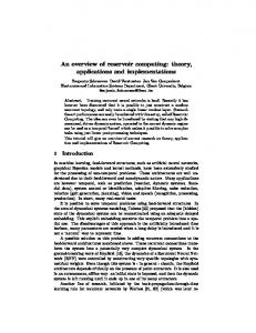
10% sparsity provides a rather robust performance, provided that the largest eigenvalues fall within the unit circle, and cover a significant fraction of the unit circle. The spectral radius of the reservoir matrix should be smaller than 1 to ensure that the network possesses the ‘echo state property’ [1], that is, that the state is eventually (after an appropriate number of iterations) only dependent of the input data and not on the initial network state. This property makes the initial state irrelevant and we set it to zero (x(0) = 0). The input weight matrix can be initialized with small values: we use random weights in [−1, 1]. The weights from input to hidden layer were done with a bias input and uniform random connections in [−1, 1]. No connections between input layer and output layer were utilized. Similarly, there are no feedback connections from the output layer to previous layers. Only the reservoir layer contains recurrent connections. Fig. 1. Representation of a reservoir network. Large circles are the neurons. The middle (blue) layer is the reservoir. Dashed connections are optional (and not used in this paper).

Figure 1 presents the general scheme of a reservoir network. Notice that the reservoir is the big layer, there can be connections directly from the input to the output layers and there can also be feedback connections from the output to the reservoir and to itself. Inside the reservoir, there are feedback connections since the neurons are randomly connected to each other. These connections are typically sparse. For the most simple case (the only recurrent connections are in the reservoir), we can write the state x(t + 1) of a N neurons reservoir at time t + 1, of an ESN with K inputs and L outputs, as: x(t + 1) = f (W x(t) + W in u(t + 1))

(1)

where f (·) is the reservoir nonlinear activation function, W is the N × N reservoir weight matrix, W in is the N × K input weight matrix and u(t + 1) is the input data. The L-dimensional network output is given by y(t) = g(W

out

x(t))

(2)

where g(·) is the output linear activation function and W out is a L × N output weight matrix. We consider g(·) to be the identity function. The way to use a reservoir network is: 1) create the random reservoir connections with a particular degree of connectivity; 2) create the input and output weight matrices; 3) feed the training data into the network and save the reservoir states for each input; 4) after having showed the complete training set to the network, find the output weights using a linear solver, given the state of the reservoir and the desired target for each input signal; 5) with the trained output layer the network can be used in test mode. The size of the reservoir, N , and the sparsity of the connections within the reservoir are meta-parameters that usually are not critical. It was found that 200 reservoir neurons with

III. R ESERVOIR COMPUTING FOR STATIC CLASSIFICATION PROBLEMS

The traditional use of reservoir computing has been to solve time dependent problems. We now discuss the adaptation necessary to use the reservoir approach on static classification problems. and can be shown to the network in any order. The index t in the equations is only used to distinguish between different patterns and no longer represents time. To ‘break’ the recurrent dependence of the state on time t on the previous state (t − 1) we propose the use of reservoir stabilization. The way this works is the following: keep each input signal present in the network input until the outputs of the reservoir neurons have almost no change. During stabilization the output layer is ignored. The state equation is iterated (upper index) until x(t + 1) does not change significantly. Notice that we do not use the activation function here. x(t + 1)(i) = W x(t)(i−1) + W in u(t + 1)

(3)

Figure 2 presents the output of the first 20 neurons of a reservoir during stabilization, for a spectral radius of 0.99. The values shown were passed through a sigmoid function for display purposes. It can be seen that the outputs oscillate but eventually stabilize. These final values are the ones considered as the state for the adaptation of the output layer. The time it takes to stabilize the state of the reservoir neurons depends on the spectral radius: the larger it gets (up to 1) the longer it takes for the dynamics to settle. Figure 3 shows the same outputs as in figure 2 (all other things being equal) but using a reservoir with a spectral radius of 0.55. The stabilization occurs within about 20 iterations as before it took around 800. The importance of the dynamics is still not clear to us. The final output layer weight adjustment can be done in several ways. Since the problem is a linear one, we can use a simple linear solver, thus no actual parameters need to be adjusted. We found that a more powerful solver can improve

Fig. 2. Output of the first 20 neurons of a reservoir during stabilization. The X axis represents the number of stabilization iterations. Spectral radius of 0.99.

Fig. 4. Haykin(2000,20) consists of 2000 unbalanced cartoon spiral data, with 400 data in the positive class and 1600 data in the negative class [12].

Fig. 3. Output of the first 20 neurons of a reservoir during stabilization. The X axis represents the number of stabilization iterations. Spectral radius of 0.55.

the results and in this paper we present results of the reservoir approach for static classification problems using PLS. IV. E XPERIMENTS We performed 25 experiments on different classification benchmark datasets (see Table I) that are challenging, nonlinear, and generally accessible and frequently cited in the literature. In the case of reservoir computing the linear solver used the classical Partial Least Squares or PLS method as discussed in [11]. PLS has the advantage of being a robust linear equation solver where just one parameter (the number of latent variables) needs to be determined. We also calculated classification results with two other powerful traditional nonlinear classification methods: Kernel Partial Least Squares (K-PLS) [8] and Least Squares SVMs or LSSVMs [9]. We also included the classification results for state-of the art neural networks with entropic error metrics as reported in the Ph.D. dissertation by Luís Silva [10]. It would be worthwhile to present other error metrics besides overall classification rates such as the balanced error ratio and the

Adjusted Rand Index (ARI), but we decided not to so in this study because the results in [10] only provide overall classification rates. The checkerboard data and the Haykin data are less conventional and deserve a brief explanation. We generated three checkerboard benchmark data binary classification problems as indicated by Check4x4(200,50), Check2x2(200,50) and Check4x4(1000,20). The 4x4 or 2x2 indicated whether we are dealing with a 2x2 or a 4x4 checkerboard. The additional info between brackets indicates the total number of data and the ratio of samples between the total number of data and the positive class. For example Check4x4(1000,20) indicates that we generated 1000 random data on a 4x4 checkerboard with 200 data in the positive class and 800 data in the negative class. Similarly, Haykin(2000,20) refers to 2000 binary unbalanced cartoon spiral data [12], where there are 400 positive samples and 1600 negative samples as shown in figure 4. All the input patterns were first standardized (i.,e., the features are scaled by subtracting their average and dividing by their standard deviation). After the reservoir outputs were stabilized we did a second standardization for the reservoir neuron outputs before applying the PLS model. Note also that while applying the PLS model the target outputs are also standardized. While we found that 12 is generally a robust first guess for the number of latent variables, the number of latent variables was tuned first for the best performance on the training data only. We used the same reservoir weights for all the classification benchmark cases reported in the paper. All the results reported in table I provide classification results based on 100 experiments for each dataset with a random 50/50 split of the data for the training and test

an heuristic formula reported in [14], according to  n  32  λ = min 1; 0.05 200 

Fig. 5. Complex eigenvalues for a reservoir with 200 neurons, 10% connectivity and weights selected from a uniform random distribution in [−0.23, 0.23].

sets. The reservoir results were obtained for a reservoir with 200 neurons, with 10% of recurrent connections chosen uniformly from a [−0.23, 0.23] uniform distribution. All experiments were performed with identical reservoir weights. We did experiment with other reservoir settings as well, and the results are qualitatively similar, provided that the radius of the complex eigenvalues is large enough, but within the unit circle and we will report on these findings in further publications. The complex eigenvalues for the reservoir settings corresponding to table I are shown in figure 5. The best results for each method are presented in bold underlined script. The first column of table I indicates the dataset and the reference for the data if the data can’t be downloaded directly from the UCI data repository [13], the second column indicates the number of classes and whether the data distributions in the various classes are balanced or not balanced. The columns with headings RES1 and RES2 are the results from reservoir computing. The number of latent variables for the RES1 results is always held fixed to 12, while the number of latent variables in the RES2 results is indicated in the column with as header LV2. The K-PLS classification results used a radial basis function (RBF) or Gaussian kernel are reported in the column headed K-PLS and the required parameter settings are the number of latent variables and the Gaussian Kernel Parzen window as reported in the column with as header LV, σ. The PLS and K-PLS methods for multi-class classification problems are performed in an orthogonal multi-output representation if the classes are categorical, otherwise a single output mode was used for multi-class classification problems. For the least squares support vector machine results we used an RBF kernel with the same kernel setting as was applied for the K-PLS method. In this case we tuned λ = 1/C with

(4)

The above formula n is the number of patterns. Past experiments have shown that above formula is generally quite robust and provides a close to optimal performance. We did check for the smaller datasets whether hand-tuning the regularization penalty factor, λ, would lead to a superior performance over the other classification methods. Note that for the Haykin(2000,20) and for the credit data we actually indicated a tie between reservoir computing and K-PLS, because the balanced error (not shown in table), which is actually more meaningful than the overall classification rate for unbalanced data, showed a better performance for reservoir computing. Note also that all LS-SVM results are for a single output mode representation for multi-class classification problems and that the results for non-ordinal multi-class classification problems are therefore generally inferior and reported in brackets. We proceeded in this way, because or LS-SVM software is geared for binary classification problems and regression problems, and cannot handle multiple output classification. From the results reported in table I we see that there often is no clear statistically significant difference between the different methods and that the results of reservoir computing with a linear solver for the second layer compares very favorably with the other nonlinear classification methods. V. C ONCLUSIONS This paper presented an extensive experimental evaluation of a reservoir approach to the classification of static patterns. We discussed a way to use the reservoir recurrent network for problems that do not depend on time. The main advantage of the proposed approach is that it has a competitive performance relative to well established methods and only needs the adjustment of a single parameter. The results on 25 commonly used benchmark data clearly show that reservoir computing for static pattern classifications presents a viable alternative to other popular nonlinear classification methods. The reservoir computing system can be considered as a neural network with a sparsely connected recurrent Hopfield layer which trains in an unsupervised mode. The innovation of our reservoir computing approach for static pattern recognition is to let the transients settle before applying a sigmoid transfer function. The weights of the second layer of the neural network are determined by a linear partial least squares method, where the number of latent variables is the only variable that needs to be tuned. Note also that for all 25 classification problem the same reservoir weights were used in the hidden layer. We are currently studying the effect of changes in the reservoir size, sparsness and spectral radius on the classification performance.

Dataset CHD2 [13] Check2x2(200,50) Check4x4(200,50) Check4x4(1000,20) Credit [13] CTG16 [15] Fischer’s iris [13] Haykin(500,50) [12] Haykin(2000,20) [12] Ionosphere [13] Liver [13] Mushroom [13] Olive [16] PB12 [17] Pima Diabetes [13] Sonar [13] Spam [13] Synthetic Ripley[18] Thyroid [13] Tic Tac Toe [13] Titanic Survival [19] Vehicle [13] Vowel [20] WDBC [13] Wine [13]

# classes 2U 2B 2B 2U 2U 10U 3B 2B 2U 2U 2U 2U 9U 4B 2U 2U 2U 2B 3U 2U 2U 4U 11B 2U 3U

# data 303 200 200 1000 690 2162 150 500 500 351 345 8124 572 608 768 208 4601 1250 215 958 2201 846 990 569 178

# variables 13 2 2 2 15 23 4 2 2 34 6 26 8 2 8 60 57 5 5 9 3 18 10 30 13

RES1 75.571 93.430 59.050 81.864 84.565 66.258 94.613 94.188 87.104 91.875 70.286 99.459 92.731 92.928 73.021 74.260 93.286 90.725 96.429 75.560 78.429 76.466 55.941 97.143 97.617

LV1 12 12 12 12 12 12 12 12 12 12 12 12 12 12 12 12 12 12 12 12 12 12 12 12 12

RES2 82.143 94.000 75.170 92.840 86.249 74.914 97.333 96.252 91.016 92.286 72.571 99.916 95.227 92.898 79.286 76.048 93.429 89.248 97.143 76.733 76.000 77.544 87.521 96.143 97.865

LV2 1 20 40 55 3 50 5 35 35 6 6 5 15 20 4 7 15 5 15 5 5 20 50 20 7

Silva[10] 83.33 92.84 79.40 84.50 88.50 70.32 94.62 92.90 76.82 79.18 93.35 96.75 81.93 88.47 97.44 98.05

K-PLS 80.441 94.370 80.770 94.642 86.461 55.169 96.507 96.106 96.760 94.858 71.347 99.568 92.427 92.645 76.794 84.548 92.111 89.288 96.744 97.962 77.619 79.187 96.733 96.469 97.157

LS-SVM 80.901 94.190 80.580 94.702 84.565 (27.139) 96.907 95.860 96.420 96.571 69.714 99.996 (85.759) (24.980) 76.628 84.346 92.947 89.560 91.184 66.543 67.599 (65.173) (59.547) 95.714 97.506

LV, σ 3,20 5,0.3 5,0.2 5,0.2 5,7 5,1 5,5 5,0.2 5,0.2 5,3 5,4 12,2 9,2 5,1 5,5 5,5 5,5 5,2 5,1 20,10 5,100 20,20 20,1.5 5,3 5,3

TABLE I E XPERIMENT RESULTS ON 25 DATASETS . RES1 AND RES2 ARE OBTAINED WITH THE RESERVOIR . B EST RESULTS ARE BOLD UNDERLINED . S EE TEXT FOR DETAILS .

R EFERENCES [1] H. Jaeger, “The ‘echo state’ approach to analysing and training recurrent neural networks,” Fraunhofer Institute for Autonomous Intelligent Systems, Tech. Rep. GMD Report 148, 2001. [2] W. Maas, T. Natschläger, and H. Markram, “Real-time computing without stable states: A new framework for neural computation based on perturbations,” Neural Computation, vol. 14, no. 11, pp. 2531–2560, 2002. [3] D. Verstraeten, B. Schrauwen, M. D’Haene, and D. Stroobandt, “An experimental unification of reservoir computing methods,” Neural Networks, vol. 20, pp. 391–403, 2007. [4] M. Skowronski and J. Harris, “Minimum mean squared error time series classification using an echo state network prediction model,” in IEEE International Symposium on Circuits and Systems – ISCAS 2006, Island of Kos, Greece, May 2006, pp. 3153–3156. [5] J. J. Steil, “Backpropagation-Decorrelation: online recurrent learning with O(N) complexity,” in Proc. IJCNN, vol. 1, July 2004, pp. 843– 848. [6] M. H. Tong, A. D. Bickett, E. M. Christiansen, and G. W. Cottrell, “Learning grammatical structure with echo state networks,” Neural Networks, vol. 20, no. 3, pp. 424–432, April 2007. [7] H. Paugam-Moisy, R. Martinez, and S. Bengio, “Delay learning and polychronization for reservoir computing,” Neurocomputing, vol. 71, pp. 1143–1178, 2008. [8] R. Rosipal and R. Trejo, “Kernel partial least squares regression in reproducing kernel hilbert space,” Journal of Machine Learning Research, no. 2, pp. 97–123, 2001. [9] J. Suykens and J. Vandewalle, “Least squares support vector machine classifiers,” Neural Processing Letters, vol. 9, no. 3, pp. 293–300, 1999. [10] L. Silva, “Neural networks with error-density risk functionals for data classification,” Ph.D. dissertation, University of Porto, Portugal, 2008. [11] S. Wold, M. Sjöström, and L. Eriksson, “PLS-regression: a basic tool of chemometrics,” Chemometrics and Intelligent Laboratory Systems, vol. 58, pp. 109–130, 2001. [12] S. Haykin, Neural Networks: A Comprehensive Foundation, 2nd edition. Prentice Hall, 1999. [13] C. Blake, E. Keogh, and C. Merz, “UCI repository of machine learning databases,” 1998, http://www.ics.uci.edu/˜mlearn/MLRepository.html.

[14] M. Embrechts, B. Szymanski, and K. Sternickel, “Introduction to scientific data mining: direct kernel methods and applications,” in Computationally Intelligent Hybrid Systems: The Fusion of Soft and Hard Computing. [15] J. Marques de Sá, Applied statistics using SPSS, STATISTICA and MATLAB. Springer, 2003. [16] M. Forina and C. Armanino, “Eigenvector projection and simplified nonlinear mapping of fatty acid content of italian olive oils,” Ann. Chem., vol. 72, pp. 125–127, 1981. [17] R. Jacobs, M. Jordan, S. Nowlan, and G. Hinton, “Adaptive mixtures of local experts,” Neural Computation, no. 3, pp. 79–87, 1991. [18] B. Ripley, Pattern Recognition and Neural Networks. Cambridge University Press, 1996. [19] R. Dawson, “The unusual episode data revisited,” Journal of Statistics Education, vol. 3, no. 3, 1995. [20] T. Hastie, R. Tibshirani, and J. Friedman, The Elements of Statistical Learning: Data Mining, Inference, and Prediction. Springer, 2001.