weights from the inputs to the reservoir and the reservoir weights are ran- domly selected. ... pattern recognition has a conventional fan-out input layer, a hidden layer with ..... Portugal, May 2008. http://www.di.ubi.pt/Ëlfbaa/entnets.html.
Reservoir computing for static pattern recognition Mark J. Embrechts1 and Lu´ıs A. Alexandre2 and Jonathan D. Linton3
∗
1 - Rensselaer Polytechnic Institute - Decision Sciences and Engineering Systems CII 5219, Troy, NY 12180 - USA 2 - University of Beira Interior - Department of Informatics and Instituto de Telecomunica¸co ˜es, Covilh˜ a - Portugal 3 - University of Ottawa - Telfer School of Management Ottawa - Canada Abstract. This paper introduces reservoir computing for static pattern recognition. Reservoir computing networks are neural networks with a sparsely connected recurrent hidden layer (or reservoir) of neurons. The weights from the inputs to the reservoir and the reservoir weights are randomly selected. The weights of the second layer are determined with a linear partial least squares solver. The outputs of the reservoir layer can be considered to be an unsupervised data transformation. This stage has a brain-like plausibility. This paper shows that by letting the dynamics of the reservoir evolve to a stable solution, and then applying a sigmoid transfer function, reservoir computing can be applied as a robust and highly accurate pattern classifier. Reservoir computing is applied to 16 difficult multi-class classification benchmark cases, and compared with the best results of state-of the art neural network classification methods with entropic error criteria.
1
Introduction to reservoir computing
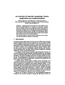
Reservoir computing [1-2] refers to a class of recurrent artificial neural networks (RANNs) consisting of liquid state machines (LSM) [3-4], echo state networks (ESN) [5], back-propagation decorrelation networks (BPDC) [6]. Reservoir computing can be based on either McCullough-Pitts neurons or spiking neurons. A simple layout for a reservoir computing based artificial neural network for static pattern recognition has a conventional fan-out input layer, a hidden layer with sparse recurrent connections and a linear output layer (with no activation function) as depicted in Figure 1. Contrary to the more traditional feed-forward or recurrent neural networks, the input weights and the feedback reservoir weights are randomly assigned. For static pattern recognition this random weight assignment is subject to the condition that the reservoir dynamics converge: i.e., ∗ Support for this research has been provided by the Canadian Natural Sciences and Engineering Research Council. We acknowledge the support of the Portuguese FCT - Funda¸c˜ ao para a Ciˆ encia e Tecnologia, POS Conhecimento and FEDER (project POSC/EIA/56918/2004).
the complex eigenvalues of the reservoir layer have to fall within the unit circle of the complex plane. Once a good reservoir is found for the hidden layer, the same reservoir weights can be used for different classification problems: i.e., the reservoir weights are conditioned rather than trained. This paper proposes a novel way for reservoir computing for static pattern recognition in the sense that the outputs of the reservoir layer are determined by applying a sigmoid-like activation function after the reservoir dynamics have stabilized. This paper is organized as follows: section 2 highlights the details of reservoir computing for static pattern recognition. Section 3 compares the results of reservoir computing on 16 challenging benchmark classification problems with the results obtained with neural networks trained with the back-propagation algorithm. Section 4 presents preliminary conclusions and remarks on the promise of reservoir computing for static pattern recognition problems.
2
Reservoir computing for static pattern recognition
Prior applications of reservoir computing were mostly limited to time series analysis applications. Reservoir computing for static pattern recognition exploits the dynamics of the reservoir layer. The activation function is applied only after the reservoir dynamics have stabilized. Note that so far the outputs from the reservoir layer are determined by an unsupervised procedure and there is no need to apply back-propagation or back-propagation through time for the hidden credit assignment problem: i.e., the reservoir can be considered as a data transform stage, and machine learning will be applied only to the transformed data. Note also that because of that reason, this paper does not consider any connections between the input layer and the output layer (or vice versa). Only the weights of the output layer are determined by a supervised process. Because the output layer has no activation function, these weights can be determined with a simple linear regression model or by applying alternate linear techniques such as ridge regression [7], principal component regression, and partial least squares regression [8]. The reservoir would typically have a few hundred neurons and the interconnections between the feedback reservoir units would be sparse (e.g., less than 10 percent connections). The weights of the input layer and the reservoir connections are selected from a uniform random distribution between zero and a maximum boundary. This maximum boundary is chosen such that oscillations after the reservoir layer stabilize. The main advantage of reservoir computing is that because the reservoir needs a robust conditioning of the weights, rather than a highly iterative training of the weights, reservoir computing does not require extensive parameter tuning, and can therefore in principle learn from fewer (or hopefully just from a few) patterns. Reservoir computing, at least as far as the input and reservoir weights are concerned, can therefore be considered as a brain-like plausible method: i.e. it is possible or plausible that similar processes take place in the brain. This last statement has to be considered in the context of the back-propagation algorithm [9]. Because the back-propagation algorithm is highly supervised and not local, it is
Fig. 1: Simple schematic of a reservoir-computing based artificial neural network for static pattern recognition (with bias weights in the input layer). Note that the transfer function in the reservoir layer is applied after the reservoir outputs have converged to stable values. highly unlikely that the brain employs a method similar to the back-propagation algorithm for pattern recognition.
3 3.1
Benchmark experiments Multi-class classification datasets
Initial experiments of static pattern recognition with reservoir computing are extremely encouraging for 16 challenging benchmark classification problems. These mostly nonlinear and multi-class classification benchmark problems were selected because they were explored at length in the dissertation of Luis da Silva [10] with extensive experiments comparing neural networks trained with the traditional back-propagation algorithm and improved neural networks using the back-propagation algorithm with an entropy based cost function. The results for these same problems were furthermore found to be comparable with those obtained by applying kernel partial least squares methods [11] and support vector machines [12], as reported in [13]. Table 1 presents a comparison between reservoir computing for static pattern recognition and the best results reported in [10] for the same datasets. 3.2
Data preprocessing and reservoir conditioning
Before showing data to the reservoir layer the variables are standardized (i.e., each variable is centered by subtracting the average column value for each variable and dividing by the standard deviation). Similarly, for the second phase of the network, the reservoir outputs are once more standardized. Note that for
the PLS classification task the targets are standardized as well. The reservoir computing part assumes a reservoir with 200 neurons, where the neurons in the hidden layer have 10 percent sparse connections. The maximum weight for the uniform random weights from input to hidden layer was set to unity, while the maximum weight for the reservoir weights was set to 0.23. The neurons used were analog. 3.3
Benchmark Results
The first column in Table 1 describes the datasets and the source for the data, where UCI stands for the University of California data repository [14]. The second column indicates the number of classes, whether the classes are balanced or unbalanced, the number of data records and the number of features. The table presents the percent correct classification because that was the only metric evaluated in [10]. All calculations reported in [10] and in this paper were based on a 50/50 training/test data split and repeated 100 times with different splits. The class distributions for the different data splits were not held equal. The reservoir computing cases use a linear partial least squares (PLS) model [8] to solve for the neural network weights of the second layer. We use PLS because it is a widely proven method in chemometrics and is generally more robust and easier to tune than ridge regression. Two results for the reservoir computing cases are reported: one (RES1) based on a choice of 12 latent variables, and a second set of results (RES2) for an optimal number of latent variables (corresponding to the column LV2). The percentage for the best results for each dataset is highlighted in bold and underscored. Note that in 50% of the cases reservoir computing gave the best results, but that the best results for reservoir computing and the best results reported in [10] are very similar for most cases. Note that all the reservoir models were evaluated with the same reservoir weights and that even though most of the benchmark classification problems listed in table I require nonlinear models for good results, only a linear model was applied to determine the weights of the second layer of the reservoir network. What is worth mentioning here is that the PLS method for determining the weights of the last layer, after the reservoir layer, now requires a much higher number of latent variables than is usually the case for PLS models. This indicates that the reservoir layer tends to spread out the eigenvalues more and that more eigenvalues are now relevant and important. This also explains why a standard regression model often yields a reasonable model for reservoir computing. Note that the results from [10] were all best case results, and were the best picks for a variety of neural network models and parameter settings. In the case of reservoir computing only the number of latent variables for the linear PLS model needs to be determined (once the reservoir settings have been conditioned). Note also that the same reservoir weights and settings were used for all 16 benchmark problems.
Dataset CHD2 [14] Check2x2(200,50) Check4x4(200,50) CTG16 [18] Ionosphere [14] Liver [14] Olive [15] PB12 [16] Pima Diabetes [14] Sonar [14] Spam [14] Thyroid [14] Vehicle [14] Vowel [17] WDBC [14] Wine [14]
#classes, #data, #vars 2U,303,13 2B,200,2 2B,200,2 10U,2162,23 2U,351,34 2U,345,6 9U,572,8 4B,608,2 2U,768,8 2U,208,60 2U,4601,57 3U,215,5 4U,846,18 11B,990,10 2U,569,30 3U,178,13
RES1 75.571 93.430 59.050 66.258 91.875 70.286 92.731 92.928 73.021 74.260 93.286 96.429 76.466 55.941 97.143 97.617
RES2 82.143 94.000 75.170 74.914 92.286 72.571 95.227 92.898 79.286 76.048 93.429 97.143 77.544 87.521 96.143 97.865
LV2 1 20 40 50 6 6 15 20 4 7 15 15 20 50 20 7
Silva [10] 83.33 92.84 79.40 84.50 88.50 70.32 94.62 92.90 76.82 79.18 93.35 96.75 81.93 88.47 97.44 98.05
Table 1: Benchmark comparisons for reservoir computing for the 16 multi-class classification data sets in [10]. The number of latent variables for RES1, LV1, is 12 in all cases.
4
Conclusions
This paper introduced reservoir computing for static pattern recognition. The novelty of this paper is that for static pattern recognition tasks, the reservoir dynamics are stabilized before applying the sigmoid activation function. We have demonstrated that reservoir computing shows excellent classification accuracy for 16 challenging nonlinear multi-class and often unbalanced classification tasks. These results are impressive because only a linear partial least squares (PLS) model was used for determining the weights of the second layer, requiring just one single parameter setting (i.e., the number of latent variables used in PLS). We have shown multi-class classification with reservoir computing for static pattern recognition is robust to the reservoir settings: (i) the same reservoir was used for all classification tasks, and (ii) preliminary experiments with 3 different reservoir settings showed qualitatively similar results. The reservoir layer performs a nonlinear data projection in an unsupervised mode and that contrary to neural networks trained with the back-propagation algorithm reservoir computing is (more) brain-like plausible. Because there is no need for extensive parameter tuning, reservoir computing also holds the promise of learning from fewer patterns. There are many open issues with reservoir computing left that need further investigation. Obvious questions are: (i) Can we condition reservoirs for certain types of pattern recognition problems? (ii) What is the role of the sparsity of the reservoir? (iii) Because reservoir computing relies on recurrent neural networks, is it possible to achieve superior results for connection problems [19]? (iv) How to condition optimal reservoir settings for such problems? (v) Is it possible to replace the PLS solver for the second layer by a more brain-like plausible algorithm? (vi) Why do PLS models require a
high number of latent variables for optimal results? (vii) Is it possible to gain a physical insight into the required number of latent variables?
References [1] D. Verstraeten, B. Scrauwen, M. D’Haene, and D. Stroobandt, An experimental unification of reservoir computing methods. Neural Networks, Vol. 20, pp. 391-403, 2007. [2] Benjamin Schrauwen, On implementing reservoir computing. Invited talk, NIPS workshop, December 8-9, Whistler, CA, 2006. [3] Wolfgang Maass, and Henry Markram, On the computational power of recurrent circuits of spiking neurons. Journal of Computer and System Sciences. Vol. 69(4), pp. 593 - 616, 2004. [4] Wolfgang Maass, Thomas Natschl¨ ager, and Henry Markram, Real-Time computing without stable states: A New Framework for Neural Computation Based on Perturbations. Neural Computation. Vol. 14, pp. 2531-2560, 2002. [5] Jaeger H., Adaptive nonlinear system identification with echo state networks. In Advances in Neural Information Processing Systems, Vol. 15, S. Becker, S. Thrun, and K. Obermayer (Eds.), MIT Press, Cambridge, MA, 2003. [6] Jochen J. Steil, Backpropagation-Decorrelation: Online recurrent learning with O(N) complexity. Proceedings IJCNN, Vol. 1, pp. 843-848, 2004. [7] A. E. Hoerl, and R. W. Kennard, Ridge regression: Biased estimation for non-orthogonal problems. Technometrics, Vol. 12, pp. 69-82, 1970. [8] Svante Wold, Michael Sj¨ ostr¨ om, and Lennart Eriksson, PLS-Regression: a basic tool of chemometrics. Chemometrics and Intelligent Laboratory Systems, Vol. 58, pp. 109-130, 2001. [9] P. J. Werbos, Beyond regression. New tools for prediction and analysis in the behavioral sciences. Ph.D. Thesis. Harvard University, 1974. [10] Lu´ıs Miguel Almeida da Silva, Neural networks with error-density risk functionals for data classification. Ph. D. Dissertation, FEUP. School of Engineering, University of Porto, Portugal, May 2008. http://www.di.ubi.pt/˜lfbaa/entnets.html [11] Rosipal R., and Trejo, L. J., Kernel partial least squares regression in reproducing kernel Hilbert spaces. Journal of Machine Learning Research, Vol. 2, pp. 97-128, 2001. [12] B. Boser, I. Guyon and V. Vapnik, A training algorithm for optimal margin classifiers. In Proceedings of the 5th Annual Workshop on Computational Learning Theory, pp. 144-152, Pittsburgh, PA, 1992. [13] Lu´ıs M. Silva, Mark Embrechts, Jorge M. Santos, and J. Marques de S´ a, The influence of the risk functional in data classification with MLPs. Proceedings of the 18th International Conference of Artificial Neural Networks, ICANN 2008. Lecture notes in computer science, vol. 5163, pp. 185-194, 2008. [14] C. Blake, E. Keogh, and C. Mertz [1988] UCI repository of machine learning databases, http://www.ics.uci.edu/˜mlearn/MLRepository.html. [15] M. Forina and C. Armanino, Eigenvector projection and simplified nonlinear mapping of fatty acid content of Italian olive oils. Ann. Chem, Vol. 72, pp. 125-127, 1981. [16] R. Jacobs, M. Jordan, S. Nowlan, and G. Hinton, Adaptive mixtures of local experts. Neural Computation, Vol. 3, pp. 79-87, 1991, [17] Trevor Hastie, Robert Tibshirani, and Jerome Friedman The Elements of Statistical Learning: Data Mining, Inference, and Prediction, Springer 2001. http://wwwstat.stanford.edu/˜tibs/ElemStatLearn/ [18] J. P. Marques de S´ a, Applied Statistics using SPSS, STATISTICA and MATLAB, pp. 420, Springer, 2007. [19] M. L. Minsky and S. A. Papert, Perceptrons. MIT Press, Cambridge, MA, 1969.