tively at all locations in an image over a discrete range of scales, using fast ...
source code for fast training of linear detectors is available1. 1.1. Contributions
..... Algorithm 1 MATLAB code for the Circulant Decomposition. Equivalent to
solving ...
2013 IEEE International Conference on Computer Vision
Beyond Hard Negative Mining: Efficient Detector Learning via Block-Circulant Decomposition Jo˜ao F. Henriques, Jo˜ao Carreira, Rui Caseiro and Jorge Batista Institute of Systems and Robotics, University of Coimbra {henriques,joaoluis,ruicaseiro,batista}@isr.uc.pt
Abstract
This type of dense search is very powerful but makes it challenging to learn the filters: learning algorithms for even the simplest models, linear classification and logistic regression, scale to ∼ 106 training examples [13]; however, a handful of test images can contain these many samples. This asymmetry between the resolution of prediction and learning has been tackled by mining for hard negative examples. In this iterative process, an initial model is trained using all positive examples and a randomly selected subset of negative examples, and this initial training set is progressively augmented with false positive examples produced while scanning the images with the model learned so far. Hard negative mining is considered expensive, and this has become less tolerable as the community has strived to scale up to a large number of object models [22]. Some recent attempts at speeding up learning have fit parametric models (Gaussians) to the background distribution [23, 18, 16], however some of these approaches are specific to particular models such as Linear Discriminant Analysis. Additionally, natural image statistics are known to be characterized by long exponential tails [26] hence may not be very faithfully represented by a Gaussian distribution. Fourier transforms have long been used to perform fast convolution, and were employed recently to accelerate detectors at test time [11]. In concurrent work, they were also used to accelerate detector training, yielding closed-form solutions for Ridge Regression [3, 20], and faster gradient computation by modifying an SVM solver [12]. A similar idea was noted earlier in image interpolation [2], but again by modifying the solver. Here we propose instead to learn directly from a training set comprising all image subwindows of a predetermined aspect-ratio and show this is feasible for a rich set of popular models including Ridge Regression, Support Vector Regression (SVR) and Logistic Regression. Intuitively, there is much redundancy in the set of all image subwindows, because of their overlap [1]. The crux of our derivation is the observation that the Gram matrix of a set of images and their translated versions, as modeled by cyclic shifts, exhibits a block-circulant structure. We demonstrate that this structure
Competitive sliding window detectors require vast training sets. Since a pool of natural images provides a nearly endless supply of negative samples, in the form of patches at different scales and locations, training with all the available data is considered impractical. A staple of current approaches is hard negative mining, a method of selecting relevant samples, which is nevertheless expensive. Given that samples at slightly different locations have overlapping support, there seems to be an enormous amount of duplicated work. It is natural, then, to ask whether these redundancies can be eliminated. In this paper, we show that the Gram matrix describing such data is block-circulant. We derive a transformation based on the Fourier transform that block-diagonalizes the Gram matrix, at once eliminating redundancies and partitioning the learning problem. This decomposition is valid for any dense features and several learning algorithms, and takes full advantage of modern parallel architectures. Surprisingly, it allows training with all the potential samples in sets of thousands of images. By considering the full set, we generate in a single shot the optimal solution, which is usually obtained only after several rounds of hard negative mining. We report speed gains on Caltech Pedestrians and INRIA Pedestrians of over an order of magnitude, allowing training on a desktop computer in a couple of minutes.
1. Introduction At the core of the most successful methods for object detection, images are scanned using learned templates. These templates may model whole objects [7], parts [14], more general mid-level fragments [4, 27] or hierarchies of filters capturing increasingly higher-level features [21]. The templates, most often HOG filters [7], are evaluated exhaustively at all locations in an image over a discrete range of scales, using fast convolution algorithms which exploit the redundancy of overlapping image subwindows. 1550-5499/13 $31.00 © 2013 IEEE DOI 10.1109/ICCV.2013.343
2760
where L is a loss function that depends on the training algorithm, and c is the regularization parameter. Many popular algorithms, including SVM, SVR, Ridge Regression and Logistic Regression can equivalently be expressed in their dual form
enables efficient learning in the Fourier domain for several loss functions, with minimal to no change required in terms of the solver (essentially using off-the-shelf solvers), and for any feature that can be implemented as a linear filter. We build on recent work that explores the circulant structure of translations in a single image [19] or in pairs (in the temporal domain) [24]. In both cases, learning is limited to Ridge Regression, while we generalize to other models such as the SVR. Additionally, while the circulant matrices used in these works model translations of one sample or a pair of samples, our block-circulant formulation allows an arbitrary number of samples. Our closed-form decomposition is simple and can be implemented with a few lines of code (Algorithm 1). Full source code for fast training of linear detectors is available1 .
n
min α
Gij = xTi xj .
1. We show that the structure of overlapping image subwindows allows efficient training of a detector with all subwindows of a set of negative images. This obviates the need for expensive rounds of hard negative mining, which only approximate the full problem. 2. A theoretical analysis of the influence of translated images over a learning problem, by proving that the resulting Gram matrix is block-circulant (Section 2).
In detection tasks, it is common to train a classifier with negative examples that are cropped from a large set of images. Although they are usually treated as i.i.d. samples [7, 14], they share an additional structure: samples from the same image are translated versions of one another. This means that overlapping pixels are constrained to be the same, resulting in a reduced number of degrees of freedom. Consider a sample x, consisting of dense features extracted inside a particular image subwindow. To simplify the discussion, assume a 1D image and a single feature, so x is an s × 1 vector; we will later show the extension to the general case is trivial. We can translate x by one element, by multiplying it with the s × s permutation matrix P , � � T 1 0s−1 , (4) P = Is−1 0s−1
4. An explicit description of the data matrix which allows the use of fast linear solvers [13], that scale linearly with the number of training examples (Sec. 4-5). Experiments show that it is possible to train with all subwindows of large training sets (INRIA and Caltech Pedestrians), achieving the same performance as several rounds of hard negative mining in a single run.
1.2. Background Learning a linear classifier is usually cast as a regularized risk minimization problem [5]. Given n samples xi and corresponding target labels yi , the goal is to find the optimal weights w,
w
1
� � L wT xi , yi ,
(3)
2. Training sets of translated samples
3. A closed-form transformation that eliminates redundant degrees-of-freedom, and simultaneously decomposes the problem into small independent subproblems (Sec. 2.2-3). The transformation is valid for several algorithms (Sec. 3).
n �
�n
The two solutions are related by w = i αi xi . Typical solvers either accept the set of samples xi (and thus can optimize the primal or dual), or accept the Gram matrix G (restricting them to the dual optimization). For datasets with many samples, the first is more advantageous. Throughout this paper, we will prove most results using the dual formulation (Section 2-3). To �avoid � creating a Gram matrix in practice, which scales as O n2 , we extend our results by presenting an explicit data matrix (Section 4). Most of the analysis is equally applicable to non-linear problems, where G is a kernel matrix [5]. However, in this paper we focus on the linear case.
The contributions of this paper are as follows.
2
(2)
with a vector α containing n dual optimization variables αi , a function D that depends on the training algorithm2 , and the n × n Gram matrix G, with elements
1.1. Contributions
min �w� + c
� 1 T α Gα + D (αi , yi ) , 2 i
where 0s−1 is a column-vector of s − 1 zeros and Is−1 is an (s − 1) × (s − 1) identity matrix. This operation is a cyclic shift: all elements are shifted one place to the right, and the element that exits the image on one side will reappear on the other side. Shifting by u elements is achieved by raising P to the uth power, P u x. Negative powers shift
(1)
i
2 Algorithms, such as the SVM, that constrain α to some set S can be i / S. dealt with easily, by defining D (αi , yi ) = ∞ if αi ∈
www.isr.uc.pt/∼henriques/
2761
(a)
(b)
(c)
Figure 1: (a) An augmented training set of n base samples, and s horizontal translations. Such data arises when training a classifier with several subwindows from images. (b) Forming the ns × ns Gram matrix G, it is clear that there is some structure at the block level. We prove G is block-circulant (Sec. 2.1). (c) Transforming by U block-diagonalizes G, resulting in s smaller and independent sub-problems (one per block). Each sub-problem corresponds to a distinct frequency of the Fourier transform.
in the opposite direction. Since P 0 is always the identity matrix, the original sample is recovered for u = 0. Our goal, then, is to train a classifier not only with a set of n samples xi , but also their translations, as modeled by cyclic shifts. In the following sections, we will consider an augmented training set X , with a total of ns samples: s translations of n base samples. Fig. 1-a illustrates this idea. � X = P u−1 xi | i = 1, . . . , n; u = 1, . . . , s .
The structure of G can be made more evident as G(u,v),(i,j) = gv−u (i, j),
which resorts to n2 auxiliary vectors g(i, j), each with s elements given by gt (i, j) = xTi P t xj .
As mentioned in Section 1.2, many learning algorithms can be expressed in the dual, in terms of a Gram matrix G. We will see how G is affected by translated samples. For the training set in Eq. 5, each row of G corresponds to a sample characterized by an index i and a translation u, and each column to another sample with index j and translation v. To deal with this fact, we will partition G into s × s blocks of size n × n. Each block (u, v) corresponds to a pair of sample translations, and each element of a block (i, j) corresponds to a pair of base samples (see Fig. 1-b). We will denote the element (i, j) of block (u, v) by G(u,v),(i,j) . Given Eq. 5, the Gram matrix is
g(i, j) = xi � xj .
(10)
Consequently, we can invoke the Convolution Theorem [17] to compute these correlations faster in the Fourier domain: g(i, j) = F −1 (F ∗ (xi ) � F(xj )) ,
(11) ∗
where � denotes the element-wise product, complexconjugation, F(·) denotes the Fourier transform, and F −1 (·) its inverse.
2.2. Block-diagonalization of G
(6)
Recall that each element of G encodes the interaction between a pair of samples from X . Intuitively, if the interactions between some groups of samples are set to 0, we can treat each group independently in subsequent computations. This is proved in Section 3. For now, we will see a transformation of G that achieves this goal. Block-diagonalization consists of finding a matrix U ¯ = U GU −1 takes block-diagonal form: such that G
Using known properties of permutation matrices [17], G(u,v),(i,j) = xTi P v−u xj .
(9)
This reveals that storing the full G (which is ns × ns) is not necessary, as only n2 vectors with s elements are required. Another advantage is that, since Eq. 9 computes dotproducts between xi and all translations of xj , it is equivalent to the correlation between vectors (denoted with �),
(5)
2.1. The structure of the Gram matrix
� �T G(u,v),(i,j) = P u−1 xi P v−1 xj .
(8)
(7)
Since the blocks (u, v) are not independent, but a function of v − u,3 G is a block-circulant matrix [8]. 3 More precisely, P v−u is a function of (v − u) modulus n, because of its cyclic nature: P kn = P 0 for all integers k.
2762
⎡ ⎢ ¯=⎢ G ⎢ ⎣
¯ G(1)
⎤ ¯ G(2) ..
.
¯ G(s)
⎥ ⎥ ⎥. ⎦
n
min α ¯f
(12)
The proof is given in Appendix A.1 (supplemental material). We now discuss the implications for a number of learning algorithms.
(13)
where ⊗ is the Kronecker product, In an identity matrix, and Fs is the s × s Discrete Fourier Transform (DFT) matrix [8]. Multiplying any vector by the DFT matrix of corresponding size is equivalent to taking its Fourier transform (Fs x = F(x)), so it is not surprising that we can block¯ ) diagonalize G purely using Fourier transforms. Each G(f block has elements [9] ¯ ij (f ) = g¯f (i, j), G
Ridge Regression. Ridge regression (RR) is a regularized form of least-squares, with loss function � � � �2 L wT x, yi = wT x − yi . (17) 1 2 αi − 1c αi yi [25]. Since its The dual has D (αi , yi ) = 2c terms are all dot-products, the decomposition is exact.
Support Vector Regression. L2 -SVR penalizes errors with the squared epsilon-insensitive loss �2 � � � � �2 L (f (x), y) = �wT x − y �� = max 0, �wT x − y � − � . (18) 1 2 αi − αi yi + � |αi | [28, The dual has D (αi , yi ) = 2c Section 6.2.2]. Only the last term, an L1 -norm, is not a dotproduct. As such, the approximation error is bounded by ¯ 1 − �α�1 |. � |�α�
(14)
¯ (i, j) = F (g(i, j)). Plugging in Eq. 11, it simplifies with g to ¯ (i, j) = F ∗ (xi ) � F(xj ). g
f = 1, . . . , s,
(16) ¯ = U α and y ¯ = U y. Both with the transformed variables α ¯ f , each with ¯ and y ¯ are partitioned into s blocks α ¯ f and y α n elements α ¯ f i and y¯f i . This relation is exact if the function D only depends on dot-products of its arguments, and approximate otherwise.
¯ ), and the remaining The s diagonal blocks are denoted G(f elements are 0. Each block is n × n. Since G is block-circulant, a closed-form solution for U exists [9]. It is given by U = Fs ⊗ In
� 1 H¯ ¯ f Gf α ¯f + α D (α ¯ f i , y¯f i ) , 2 i
(15)
3. Separability of learning problems
The general case. The same analysis applies to L1 -SVR, Logistic Regression and other dual formulations, with varying degrees of approximation. It is also possible to characterize the transformations that preserve L1 and L2 -norms exactly, but such a restriction makes them less useful (this is explored in Appendix A1.1). We do not use SVM because it restricts the labels to {−1, 1}, and a unitary transformation would fall outside this set.
We now need to prove the intuition that the blocks of a ¯ indeed represent indepenblock-diagonal Gram matrix G dent learning problems. This can yield considerable computation and storage savings, since the number of elements under consideration is (s − 1) s times smaller than for the full G. The exact partitioning into sub-problems is also suitable for parallel implementations that take full advantage of modern architectures. At this point, it is important to point out that the transformation matrix U we used in Section 2.2 is unitary. This implies that U −1 = U H , where (·) H is the Hermitian transpose (transposition and complex-conjugation).4 The interest in unitary transformations lies in the fact that ¯ = U b, then ¯ = U a and b they preserve dot-products: if a ¯ = aH b. Because L2 -norms are dot-products, they are ¯H b a 2 2 also preserved: aH a = �a� = �¯ a� .
4. Explicit data matrix The transformed Gram matrix for each of the s sub¯ ), can be used directly in a dual solver (e.g., problems, G(f libsvm [13]). However, if n is large, an explicit description of the transformed data matrix that generates such a Gram matrix (through Eq. 3) would be more desirable. By inspecting Eq. 14-15, it can be seen that each block ¯ ) corresponds to a distinct Fourier frequency f , and G(f each of its elements (i, j) is simply the product of frequency f of the Fourier transforms of samples xi and xj . Because it is a simple product, it can be factorized into
¯ = Theorem. Given a unitary matrix U such that G −1 ¯ is block-diagonal, with s blocks Gf , then Eq. 2 U GU can be decomposed into the s sub-problems 4 The Hermitian transpose is the most natural extension of transposition to the complex domain, simplifying many expressions. In fact, many numerical packages such as MATLAB use it as the default transposition operator. This has no effect over real matrices.
¯ ) = X(f ¯ )X ¯ H (f ), G(f
2763
(19)
where c is the regularization parameter (Section 1.2). The only difference from the real case is that the solution must be complex-conjugated. Ridge Regression usually performs only slightly worse than SVR in many tasks, so it is useful as a validation for more complicated approaches [25] . The SVR can deal with the complex case by extending its loss function (Eq. 18) from the real line to the complex plane:
Algorithm 1 MATLAB code for the Circulant Decomposition. Equivalent to solving a regression with all spatial translations of the given samples. The independent regression sub-problems can be solved in parallel. The full test suite can be downloaded at: www.isr.uc.pt/∼henriques/
Inputs: • X (m features on a s1 × s2 grid for n samples, total size s1 × s2 × m × n) • Y (labels, size s1 × s2 × n) • regression (a linear regression function) Output: • W (weights, size s1 × s2 × m)
� � � ��2 � � ��2 � L wH x, y = �Re wH x − y �� + �Im wH x − y �� , (21) where Re (·) extracts the real part of a complex number, and Im (·) the imaginary part. For real arguments, this reduces to the simple SVR. We can prove (Appendix A.2) that this is equivalent to a simple SVR with the augmented data matrix X � and augmented targets y� ,
X = fft2(X) / sqrt(s1*s2); Y = fft2(Y) / sqrt(s1*s2); Y(1,1,:) = 0; X = permute(X, [4, 3, 1, 2]); Y = permute(Y, [3, 1, 2]); for f1 = 1:s1 for f2 = 1:s2 W(f1,f2,:) = regression( ... X(:,:,f1,f2), Y(:,f1,f2) ); end end W = real(ifft2(W)) * sqrt(s1*s2);
�
X =
Re (X) Im (X)
Im (X) −Re (X)
� ,
�
y =
�
Re (y) Im (y)
� ,
(22) and the complex solution w can be reconstructed from the augmented real solution w� , � � Re (w) � w = . (23) Im (w)
¯ ) is an n × 1 vector with the Fourier frequency where X(f f of each sample. This explicit description of the data ¯ ) allows us to use a fast primal solver such as matrix X(f liblinear [13].
Note that this is not the same as simply concatenating the real and imaginary parts as features. The structure of X � ensures that the properties of complex numbers are respected (e.g., i.i = −1, with i the pure-imaginary unit).
Extension to two dimensions. All properties of the Fourier transform (FT) and block-circulant matrices we used have direct equivalents in 2D, i.e., when samples contain s1 × s2 spatial cells. We just have to replace the 1D FT with the 2D FT, and set s = s1 s2 .
6. Experiments We tested the proposed decomposition on a number of detection tasks. Recall that our method replaces the traditional hard negative mining steps with a single learning phase. As such, the goal of these experiments is not to show greater accuracy, but to verify that we can achieve accuracy that is competitive with several rounds of hard negative mining, all other components being constant. If we introduced different variations (features, etc), results would be less conclusive. We chose the task of learning a single HOG filter from full object exemplars, which captures the core component shared by most modern object detectors [14, 4]. Note that our contribution is orthogonal to other recent advances in object detection, such as the use of part filters and multiple object components [14, 4, 27]. In our tests, we will apply the Circulant Decomposition (CD) to an SVR solver, as we found SVR to perform similarly to regular SVM in practical object detection tasks. The experiments will evaluate several aspects: 1) how detection performance with the CD single-batch learning relates to SVM learning as the number of rounds of hard negative
Extension for multiple features per cell. We can simply ¯ ) to be a n × m matrix with the Fourier freextend X(f quency f of m features. By additivity of the dot-product, the Gram matrix obtained this way is the sum of Gram matrices over all m features, and all properties are preserved.
5. Complex-valued regression The fact that the data matrices of Eq. 19 are complex may apparently present some difficulties, since regression is usually real-valued. In this section we discuss some solutions. We consider a generic data matrix X and regression targets y. The simple algorithm of Ridge Regression is already prepared to deal with complex values: � �−1 H X y, w∗ = X H X + c−1 I
�
(20) 2764
per: that a Circulant Decomposition is equivalent to training with all negative windows, a feat that can only be approximated by several rounds of hard negative mining. Fig. 2 shows a comparison of CD and different numbers of hard negative rounds for INRIA Pedestrians and Fig. 3 shows the same comparison for the Caltech Pedestrian Detection Benchmark. Average Precision (AP) is shown in brackets. The results suggest that the Circulant Decomposition performs on par with the slower and intrinsically less complete process of learning with hard negative mining.
1
0.8
Recall
0.6
0.4 Circulant (0.805) Mining, 0 rounds (0.749) Mining, 1 rounds (0.785) Mining, 2 rounds (0.794) Mining, 3 rounds (0.796)
0.2
0
0
0.1
0.2
0.3
0.4 0.5 Precision
6.1.1 0.6
0.7
0.8
0.9
We followed the original implementation of the HOG pedestrian detector [7]. On INRIA Pedestrians the baseline classifier is trained with 12180 random negative windows, before mining hard negative examples from the set of 1218 negative images, which contains ∼ 108 potential windows. For our method, which can train with all ∼ 108 windows in this set, we consider a total of ∼ 105 base samples. The finer translations within each patch are implicitly dealt with by the Circulant Decomposition, which is the main advantage of our approach. We proceed similarly on the “reasonable” subset of the Caltech Pedestrian dataset, composed of 4250 training images obtained every 30 frames, of which 2217 are negative images, without pedestrians. All tests were done on a quad-core 3.0Ghz desktop computer. Both CD and mining implementations are parallelized, providing a fair representation of a modern set-up. An implementation of the proposed method using this data matrix is given in Algorithm 1. For HOG descriptors, m is the number of orientation bins, over an s1 × s2 grid. The indexing operations to make each sub-problem work on a different Fourier frequency f are performed by the built-in √ function permute. The factors s1 s2 are needed because most FFT implementations are only unitary if corrected by this scalar factor. Recall that s = s1 s2 when generalizing from one to two-dimensions (Section 4). Additionally, we verified experimentally that it is necessary for the regression targets to have no DC component (line 3 of Algorithm 1.) A possible reason is that the DC component of the data, which corresponds to the mean in the spatial domain, tipically has values several orders of magnitude larger than the remaining frequencies. Modeling this effect properly may lead to better performance, but will be left for future work.
Figure 2: Performance on the test set of INRIA Pedestrians using a HOG detector. It takes several rounds of hard negative mining to converge to the same results of the proposed Circulant Decomposition, which is trained on the full set of negative windows. The Circulant Decomposition allows training on the full set in one go. (AP is shown in brackets.) 1 Circulant (0.38) Mining, 0 rounds (0.165) Mining, 1 rounds (0.268) Mining, 2 rounds (0.365) Mining, 3 rounds (0.368)
0.8
Recall
0.6
0.4
0.2
0
0
0.1
0.2
0.3
0.4 0.5 Precision
0.6
0.7
Implementation
0.8
Figure 3: Performance on the test set of the Caltech Pedestrians Detection Benchmark (AP is shown in brackets) using a HOG detector. The Circulant Decomposition is competitive with 3 expensive rounds of hard negative mining.
mining increases, 2) the implicit ability of CD to enlarge the training set with many translations, and its impact on datasets with few positive samples and 3) the computational savings of CD, compared to hard negative mining, which is generally considered expensive.
6.1.2
6.1. Pedestrian detection
Cyclic shifts as a model for translation
Since samples must have the same support as the learned template w, cyclic shifts of a template-sized sample are less accurate for large translations, due to wrap-around effects. Thus in practice we collect base samples xi from negative images in a grid, at regular intervals of 2/3 of the template
We experimented with pedestrian detection on two standard datasets: the well-known INRIA Pedestrians [7] and the recent Caltech Pedestrian Detection Benchmark [10]. We will jump straight away to the main point of our pa-
2765
159
312
463
35
0.749 0.785 0.794 0.796
1
0.5 Circulant (0.805) Full SVM (0.748)
0.805 0
12
646
1272
1901
0.165 0.268 0.365 0.368
Average precision
7
3
Circulant 0 Recall
INRIA
0
Caltech
Rounds Time (s) AP Time (s) AP
Mining 1 2
139
0
0.2
0.4 0.6 Precision
(a)
0.380
0.8
0.8 0.6 0.4 0.2 0
0
0.5
1 σ
1.5
2
(b)
Figure 4: INRIA Pedestrians. (a) Comparison of Circulant Decomposition and a full SVM (not decomposed) using the same base samples. (b) Performance as spatial bandwidth σ is varied (see text). Small values offer better performance because high localization in detection tasks can be understood as suppressing off-center detections.
Table 1: Performance and timing of the proposed method on the INRIA and Caltech Pedestrians datasets, and the classical approach using increasing numbers of hard negative mining rounds. The proposed method converges on the solution in one go, requiring much less time than even a single round of mining.
size, which accounts for large translations. We verified experimentally that there is little impact in performance if we assume cyclic shifts are accurate up to ∼1/3 of the template size in all directions. The cyclic shifts P u−1 xi model the finer translations, which comes at no additional cost when using the Circulant Decomposition. This allows us to effectively model a sliding window, while collecting only a few dozen base samples per negative image. To verify that the gain in performance is truly due to the Circulant Decomposition and not the grid sampling scheme, we trained a full SVM classifier with the same base samples. The results in Fig. 4-a show that performance drops significantly without the proposed decomposition, which also makes training faster and easier to parallelize.
6.2. ETHZ Shapes As mentioned earlier, translations of positive samples are also considered. It is possible that these “virtual samples” help regularize the solution in settings with a scarcity of positive samples. To test this hypothesis, we followed the same methodology as before but on the ETHZ Shapes dataset [15]. This dataset has only between 22 and 45 positive examples for each of its 5 categories (Mugs, Bottles, Swans, Giraffes and Apple Logos), evenly split into training and testing sets. Unlike on the pedestrian detection benchmarks, where positive examples abound, here results are markedly improved using the proposed method, as visible in Fig. 5. We conjecture, based on these results, that our approach could also benefit applications such as one-shot learning and transfer learning.
6.1.3 Positive samples
7. Conclusion
Another aspect of our method is that we must choose labels for translations of positive samples, since they are implicitly accounted for during training. A translation of a positive sample at some point becomes a false positive, so a simple choice is to assign it the label +1 if t = 0 (aligned), and -1 if t �= 0 (misaligned). Alternatively, and taking advantage of the fact that regression allows labels outside the set {−1, +1}, we can use a Gaussian function to interpolate smoothly between the two, according to a Gaussian bandwidth σ. For σ = 0 the function looks like a single peak, and we recover the first choice we mentioned. This function plays a similar role to the training output plane in correlation filters [19, 3]. Performance on INRIA Pedestrians as this parameter varies is shown in Fig. 4-b. Larger bandwidths seem to degrade performance, and the best performance is attained near σ = 0. Since good localization (suppressing misaligned detections) is important in detection tasks, this result agrees with intuition.
Supported by the observation that the Gram matrix of the set of training images and their translations is blockcirculant, we have derived a closed-form decomposition that allows for popular filter-based detectors to be efficiently learned from all subwindows with fixed aspect-ratio extracted over predefined scales, in a single batch, on datasets with a few thousand training images. This is surprising since the number of subwindows is in the order of 108 , which seems to even preclude loading the data into the computer’s memory, but is feasible using our proposed embedding of the learning problem into the Fourier domain. Our methodology is likely to have broad applicability, as it allows for both a much more efficient and more complete learning process than iterative hard negative mining, used for learning virtually all modern object detectors. As future work we plan to extend our experiments beyond single-HOG detectors, and learn the types of filter collections employed by current state-of-the-art object de-
2766
Applelogos
0
0.5 Precision
1
0
0.5 Precision
1
0.5 0
Mugs
1 Recall
0.5 0
Giraffes
1 Recall
Recall
Recall
0.5 0
Bottles
1
0
0.5 Precision
1
1 Recall
Swans 1
0.5 0
0
0.5 Precision
1
0.5 0
0
0.5 Precision
1
Circulant (0.719) Mining, 3 rounds (0.596)
Figure 5: Performance on ETHZ Shapes, a dataset with scarce training data (between 22 and 45 positive examples per class, with an equal train-test split). In addition to allowing models to be trained faster, the Circulant Decomposition achieves higher performance in this case, perhaps due to the implicit inclusion of translated positive samples. (Mean AP is shown in brackets.)
tectors [14, 4]. We believe prior knowledge such as invariance is essential for efficient visual learning and are currently investigating avenues to broaden the proposed translation machinery to small in-plane rotations and local shape deformations [6].
[13] R.-E. Fan, K.-W. Chang, C.-J. Hsieh, X.-R. Wang, and C.-J. Lin. LIBLINEAR: A library for large linear classification. Journal of Machine Learning Research, 2008. 1, 4, 4, 4 [14] P. F. Felzenszwalb, R. B. Girshick, D. McAllester, and D. Ramanan. Object detection with discriminatively trained partbased models. TPAMI, 2010. 1, 2, 6, 7 [15] V. Ferrari, L. Fevrier, F. Jurie, and C. Schmid. Groups of adjacent contour segments for object detection. TPAMI, 2008. 6.2 [16] M. Gharbi, T. Malisiewicz, S. Paris, and F. Durand. A gaussian approximation of feature space for fast image similarity. In MIT CSAIL Technical Report, 2012. 1 [17] R. M. Gray. Toeplitz and Circulant Matrices: A Review. Now Publishers, 2006. 2.1, 2.1 [18] B. Hariharan, J. Malik, and D. Ramanan. Discriminative decorrelation for clustering and classification. In ECCV, 2012. 1 [19] J. F. Henriques, R. Caseiro, P. Martins, and J. Batista. Exploiting the circulant structure of tracking-by-detection with kernels. In ECCV, 2012. 1, 6.1.3 [20] H. Kiani, T. Sim, and S. Lucey. Multi-channel correlation filters. In ICCV, 2013. 1 [21] A. Krizhevsky, I. Sutskever, and G. Hinton. Imagenet classification with deep convolutional neural networks. In NIPS, 2012. 1 [22] T. Malisiewicz, A. Gupta, and A. A. Efros. Ensemble of exemplar-SVMs for object detection and beyond. In ICCV, 2011. 1 [23] M. Osadchy, D. Keren, and B. Fadida-Specktor. Hybrid classifiers for object classification with a rich background. In ECCV, 2012. 1 [24] J. Revaud, M. Douze, C. Schmid, and H. Jegou. Event retrieval in large video collections with circulant temporal encoding. In CVPR, 2013. 1 [25] R. Rifkin, G. Yeo, and T. Poggio. Regularized least-squares classification. NATO Science Series, 2003. 3, 5 [26] D. L. Ruderman and W. Bialek. Statistics of natural images: Scaling in the woods. In NIPS, 1993. 1 [27] S. Ullman, M. Vidal-Naquet, and E. Sali. Visual features of intermediate complexity and their use in classification. Nature neuroscience, 2002. 1, 6 [28] V. Vapnik. The nature of statistical learning theory. Springer, 2000. 3 [29] A. Vedaldi and B. Fulkerson. VLFeat: An open and portable library of computer vision algorithms. http://www. vlfeat.org/, 2008.
The authors would like to thank the anonymous referees for helpful suggestions. This work was supported by FCT project PTDC/EEA-CRO/122812/2010, grants SFRH/BD75459/2010 and SFRH/BD74152/2010.
References [1] B. Alexe, V. Petrescu, and V. Ferrari. Exploiting spatial overlap to efficiently compute appearance distances between image windows. In NIPS, 2011. 1 [2] D. Anguita, A. Boni, and S. Pace. Fast training of support vector machines for regression. In IEEE-INNS-ENNS International Joint Conference on Neural Networks, 2000. 1 [3] V. N. Boddeti, T. Kanade, and B. V. K. V. Kumar. Correlation filters for object alignment. In CVPR, 2013. 1, 6.1.3 [4] L. Bourdev, S. Maji, T. Brox, and J. Malik. Detecting people using mutually consistent poselet activations. In ECCV, 2010. 1, 6, 7 [5] N. Cristianini and J. Shawe-Taylor. An introduction to support vector machines and other kernel-based learning methods. Cambridge university press, 2000. 1.2, 1.2 [6] M. D. Zeiler and R. Fergus. Stochastic pooling for regularization of deep convolutional neural networks. In International Conference on Learning Representations, 2013. 7 [7] N. Dalal and B. Triggs. Histograms of oriented gradients for human detection. In CVPR, 2005. 1, 2, 6.1, 6.1.1 [8] P. J. Davis. Circulant matrices. American Mathematical Soc., 1994. 2.1, 2.2 [9] T. De Mazancourt and D. Gerlic. The inverse of a blockcirculant matrix. IEEE Transactions on Antennas and Propagation, 1983. 2.2, 2.2 [10] P. Doll´ar, C. Wojek, B. Schiele, and P. Perona. Pedestrian detection: An evaluation of the state of the art. TPAMI, 2012. 6.1 [11] C. Dubout and F. Fleuret. Exact acceleration of linear object detectors. In ECCV, 2012. 1 [12] C. Dubout and F. Fleuret. Accelerated training of linear object detectors. In CVPR Workshop on Structured Prediction, 2013. 1
2767