Sample-efficient Reinforcement Learning via Difference Models Divyam Rastogi∗,1 , Ivan Koryakovskiy∗,2 and Jens Kober3
Abstract— To render learning controllers feasible for real robots, interaction time with the real environment needs to be minimized. One of the popular approaches to tackle this is to model and improve the simulation gap. In this paper, we develop an iterative model learning approach which learns the simulation gap. Our approach provides two benefits: (1) it can scale to systems with highly non-linear and contactrich dynamics with continuous state and action spaces and (2) provide sample complexity results. The approach reduces the demand for real samples by only learning the difference in regions of the state space which are essential for completing the task. We test our approach in simulations on two platforms, an inverted pendulum and a 7-DoF walking robot. We compare the performance of the proposed approach against cold-started and warm-started learning and show the reduction of real interaction time by about 20 and 5 times, respectively.
I. I NTRODUCTION Learning with no or little prior knowledge about the environment is becoming more popular among control researchers. The reason is that learning provides a generic toolbox for solving complex high dimensional tasks possibly subject to discontinuities. A good example of such task is bipedal locomotion. The intrinsic vulnerability of bipedal walking platforms limits the amount of possible real experience, thereby making it very expensive to obtain. Therefore, data-driven methods require the development of measures which reduce their sample complexity and speed up the learning. The consequence is that such methods lack generality and hence become applicable to specific types of robots [1], [2]. In the light of the recent success of deep reinforcement learning (RL) methods for control of high degrees of freedom (DoF) systems [3], [4], we study the applicability of neural network representations to learning control policies for such systems in the real world. The methods demonstrate remarkable performance on highly challenging 3D locomotion tasks but require a large number of training samples and are therefore limited to simulated environments [5]. Furthermore, due to the discrepancy between the model and the real system, the simulation gap, policies that perform optimally in simulation fail to perform adequately in the real world, even if applied to low DoF systems like the inverted pendulum. There has been a large body of work which belong to the class of model-based RL methods which tackle the issue of high sample complexity. In these methods, the policy training *The first two authors contributed equally to this work.
[email protected], {i.koryakovskiy, j.kober}@tudelft.nl 1 Robotics
and Biology Lab, TU Berlin of BioMechanical Engineering, TU Delft 3 Cognitive Robotics Department, TU Delft 2 Department
is either interleaved with a forward model learning [6], [7] or it is done concurrently [8]. These methods usually start with no knowledge about the model and aim for learning it by interaction with the real system. However, usually an idealized model of the physical system is known but various uncertainties do not allow achieving optimal performance of the policy trained on this idealized model. To correct the discrepancy between the system and the model, [9], [10] learn the inverse model directly from the physical system. These methods assume that the inverse model can connect successive states prescribed by the nominal controller. The approach taken in [11] is free from this assumption because it learns an additive component of the forward model. The approach allows to compensate both parametric and structural uncertainties, but cannot scale to systems with discontinuities. A similar approach was proposed in [12]. Unfortunately, it uses Gaussian processes for modeling the simulation gap which limits its application to high DoF systems [3]. The approach proposed in [13] scales to high DoF systems and environmental discontinuities but requires expert guidance to select parameter sets to investigate after each model update. Approach [14] works in combination with nonlinear model predictive control which allows it to provide safety barriers on RL exploration depending on the severity of the mismatch. The approach can scale to high DoF systems with parametric and structural uncertainties but requires an additional controller at hand. In this article, our contribution is twofold. First, we propose an iterative model learning approach which scales to high DoF contact-rich systems and does not require human supervision. We assume that an idealized model of a system is provided and that the real system resembles the model to some extent. We approximate the difference with a deep neural network (DNN) which allows us to apply our method to high dimensional continuous systems. We expect that the accurate representation of the difference between systems can mitigate the simulation gap. Second, we provide a detailed sample complexity analysis by comparing the performance of our method against warm-started and coldstarted (from scratch) learning on two simulated examples: 1-DoF inverted pendulum and 7-DoF bipedal robot Leo. To our knowledge, such analysis is currently missing in the literature. Since the simulation gap only matters in regions of the state space explored by the policy, the difference model only needs to be accurate in those parts of the state space. This helps us to reduce sample complexity further since the model only needs samples in regions which are important for the task.
sk Agent rk
sidl k+1
Reward Fig. 1.
Learn policy µidl
Difference model
ak
i≤I yes
d(sk , ak ) System
Stop
Run policy on the true model to collect transitions
Proposed framework.
Update d(s, a) II. R EINFORCEMENT LEARNING We consider a standard reinforcement learning problem formulation. The learning is formalized by Markov decision process which is the tuple hS, A, T, Ri, where S is a set of ns -dimensional states s ∈ Rns , A is a set of na -dimensional actions a ∈ Rna , T : S × A × S → [0, 1] is a transition function which defines a probability of ending up in state sk+1 after taking action ak in state sk . Here k denotes discrete timesteps of the system. Reward function R : S ×A×S → R gives a scalar reward r(sk , ak , sk+1 ) for particular transitions between states. The goal of the learning agent is to maximize the discounted expected return (∞ ) X γ i Gk = E γ r(sk+i , ak+i , sk+i+1 ) (1) i=0
where γ ∈ [0; 1) is the discount factor which ensures integrability of the infinite sum. The control policy, or the actor, µ : S → A is a deterministic function which selects action ak in state sk . Exploration is achieved by adding random noise sampled from some process N . When solving continuous control problems, it is convenient to evaluate the quality of the policy by the action-value function Qµ : S × A → R, or critic. It describes the expected return after taking an action ak in state sk and thereafter following policy µ. We use a particular realization of RL, the off-policy Deep Deterministic Policy Gradient (DDPG) algorithm [3] with deep neural network function approximation and compatible features, chosen for its ability to optimize continuous control policies for high DoF systems. The value function and policy are parametrized by the network weights θQ and θµ . III. P ROPOSED METHOD A. Notation In this article, we work only with simulated models. Therefore, we create two models called idealized and true. We assume the same state space in the idealized and true models. However, inaccuracies due to the modeling differences give rise to the differences in transition probabilities. Our method minimizes the gap between these models by learning the difference model. Schematically, the proposed method is shown in Figure 1. The idealized model f idl (sk , ak ) = sidl k+1 is a forward dynamics (usually first principles) model based on a certain idealized configuration of the robot. We denote the policy trained on this model as µidl .
Learn new policy µd Fig. 2.
Algorithm overview.
The true model f true (sk , ak ) = strue k+1 is a forward dynamics model based on the real configuration of the robot. The corresponding policy trained on this model is denoted as µtrue . idl The difference model d(sk , ak ) = strue k+1 − sk+1 predicts the difference in the transition states given an initial state and action. The policy trained using the difference model is denoted as µd . B. Algorithm An overview of the algorithm is presented in Figure 2. The algorithm starts by pre-training the initial policy µidl and the corresponding value function using the idealized model of the robot. The policy behaves sub-optimally when applied to the true model due to the simulation gap. To eliminate the gap, we propose an iterative approach which consists of three distinctive steps. In the first step, we collect a number of real samples through interaction with the true model and save them in buffer D. In the second step, we use the whole buffer to learn the difference model represented by the deep neural network. The difference model predicts the difference in states between the idealized model and the true model. In the third step, DDPG is used to learn a new policy µd with this difference model. The newly obtained policy is likely to perform better on the true model. However, if the initial simulation gap is large, the new policy may still not perform satisfactory. Thus, we iterate the process of updating the difference model and the policy until a certain number of iterations is reached. To keep the successive DDPG training time short, we bootstrap parameters of the policy and the value function from the ones used in the previous iteration. C. Training data The data used for training the difference model is obtained by running the previously obtained policy on the true model µ several times. Let this policy be denoted by µ(s; θi−1 ). The µ action to be taken is calculated as a = µ(s; θi−1 ) + N . The particular advantage of using policy from the previous iteration is that it progressively matches the distribution of training transitions to those required for the successful completion of the task. Since DDPG is used to learn a new policy after every update of the difference model, the replay
buffer from the first update of the policy is saved and used in every following update. This helps to reduce the number of iterations required to find a good policy at each step and increases the diversity of samples.
φ m
IV. E XPERIMENT DETAILS
l
A. Inverted pendulum Figure 3 shows the inverted pendulum of mass m = 0.055 kg which rotates around the fixed point O located l = 0.042 m away from the center of mass of the pendulum. The ˙ is composed of pendulum angle φ pendulum state s = (φ, φ) ˙ The control input a ∈ [−3 V, 3 V] is and angular velocity φ. the voltage applied to the motor located at O. The voltage is bounded to prevent the pendulum from performing a swingup in one go. The pendulum is initialized in state s0 = (π, 0), and the agent has to learn to swing up the pendulum and balance it until the end of the 20 s episode. The reward function is given by r = −5φ2 − 0.1φ˙ 2 − 0.01a2 . Sampling period is Ts = 0.05 s. The true model has a higher pendulum mass shown in Table I. B. Bipedal robot Leo Leo [15] is a 2D bipedal robot developed by the Delft BioRobotics Lab shown in Figure 4. The robot is attached to a boom which prevents it from lateral falls. Leo is modeled using Rigid Body Dynamics Library [16] with the boom mass added to the torso. Leo has 7 actuators, two for each hip, knee, and ankle, and the last one for the shoulder. All joints and the torso-toboom connection are equipped with encoders which provide real-time measurements. The learning state space of Leo comprises of 18 dimensions which consist of the angles φ and the angular velocities φ˙ of all but shoulder joints, and the torso linear positions and velocities. The action space of Leo consist of voltages applied to each actuator except the shoulder which is actuated using a proportional-derivative controller. The reward function awards the agent 300 m−1 for every meter of forward movement of the robot. The agent is penalized by a −1.5 additional reward for every time step and by a −2 J−1 reward for every Joule of electrical work done. Premature termination of the 20 s episode due to a fall is punished by the negative reward of −75. Sampling period is Ts = 0.03 s. The true Leo model has higher torso mass and viscous friction added to all actuators. These differences affect the performance of the idealized policy when applied to the true model, occasionally leading to oscillations and eventual fall of the robot. The change in parameters is shown in Table I. C. Training data and parameters All parameters are kept the same for both systems. The DDPG critic and actor networks consist of 2 hidden layers with 300 and 400 neurons, respectively. Learning rates of
O Fig. 3.
Inverted pendulum. Fig. 4.
Leo: the model and the real robot.
TABLE I D IFFERENCE IN PHYSICAL PARAMETERS BETWEEN IDEALIZED AND TRUE MODEL . Parameter
Idealized model True model
Inverted pendulum Pendulum mass m (kg)
0.055
0.090
Robot Leo Torso mass (kg) Viscous friction coefficient (N s m−2 )
0.942 0.000
1.250 0.030
0.001 and 0.0001 are chosen for the critic and the actor. Additional parameters include a target network update rate of 0.001 and the discount rate γ = 0.99. Exploration is achieved by an Ornstein-Uhlenbeck noise model with parameters σ = 0.12 and θ = 0.15 used during warm-start learning and learning with the difference model. For cold-start learning noise parameters are slightly higher. The difference model consists of 3 hidden layers with 400 neurons in each layer. The activation function for each of the hidden layers is ReLu while the output layer has a linear activation function. To reduce over-fitting to the training data, we use dropout [17] with probability 0.3. Dropout is only applied to the hidden layers and is the same for all layers. Before each model update, 3750 data-points are collected by running the previously obtained policy on the true model which are saved to a buffer that has not limits on size. We train the network using AdaGrad [18] which is a variant of stochastic gradient descent. The advantage of using AdaGrad over normal stochastic gradient is the ability to adapt the learning rates based on the training data. This implies that the initial learning rate does not have much impact on the performance of the algorithm. D. Evaluation measures For quantitative assessment, we evaluate performance of the proposed method in terms of the undiscounted return (1). Additionally, for the Leo robot we evaluate the walked distance L and the motor work E normalized to the walked distance given by E=
J Ts X Uj − Kτ φ˙ j Uj L j=1 R
where Uj is the voltage applied to the motor j, Kτ is the motor’s torque constant, R is the winding resistance, and J is the number of learned controls.
For qualitative assessment, we also show system trajectories obtained by each method.
5000
Policy µd
Policy µidl
Return, G1
0
V. R ESULTS A. Inverted pendulum
−5000 −10000 −15000 0
1
2 3 Difference model updates
4
Fig. 5. Comparison of results by evaluating the performance of different policies on the true model for the inverted pendulum.
ϕ˙ (rad s−1 )
ϕ (rad)
Policy µtrue
a (V)
Figures 5 and 6 show the return and final trajectories obtained by the policies evaluated on the true model. The policy trained on the idealized model is not capable of balancing the pendulum and therefore obtains the lowest return of −15508. On the contrary, the proposed method of learning the difference model can evade the simulation gap. After one model update, the policy reaches the return of −660.0 which is similar to the one obtained by the policy µtrue trained on the true model. This number of updates corresponds to 3.125 min of interaction with the true model. The cold-started method requires around 75 min to converge. We also see the similarity in the final state and control trajectories in Figure 6 between policies µtrue and µd Table II compares results of learning on the true model obtained by DDPG learning from scratch (cold start), initializing the value function and the policy by learning on the idealized model (warm start) and by the proposed method. Given that we have a limit of 15000 on true model samples, the proposed method obtains the highest return. Alternatively, it requires 6 times fewer samples than the warm-started learning to reach the target return of −1000.0.
Policy µtrue
Policy µd
Policy µidl
6 3 0 30 0 −30 3 0 −3 0.0
0.5
1.0
1.5
2.0 2.5 Time (s)
3.0
3.5
4.0
Fig. 6. State trajectories and control input for policies learned on different models and evaluated on the true model.
B. Bipedal robot Leo The results of learning the policy with the difference model are presented in Figure 8. Here all policies are evaluated on the true model. Initial updates of the difference model show a high standard error, which is reduced in later updates. After 7 updates, the proposed method reaches the mean return of 2297.46 which is within 10 % of the return obtained by learning directly from the true model. This number of updates corresponds to about 13 min of interaction with the true system, while the cold-started method requires 200 min to converge. The corresponding final performance of policies evaluated on the true model is shown in Table III. In both benchmarks, the policy trained on the idealized model performs the worst. The policy µtrue provides 38.3 % improvement in the walked distance (see Figure 7) and 4.8 % reduction in the energy consumption as compared to the policy µidl . Visually, all trajectories display some irregularity of the walking cycle. As expected, the µidl policy performs worst, and its gait exhibits small step sizes and a tendency to lift the swing knee very high1 . This results in a slow walking gait. The difference model improves the idealized model. Therefore, the µd policy leads to a higher walking speed due to the reduction of the swing knee lifts. Table IV compares sample complexity results for Leo. Compared to the inverted pendulum, we increase the number of true model samples to 33750. The proposed method obtains the highest return. Alternatively, it requires about 1 Video
Link: https://youtu.be/rVIpd0qtaWA
5 times fewer samples than the warm-started learning to reach the target return of 2300. Compared to the coldstarted learning, the proposed method requires 20 times fewer samples to reach the target. VI. D ISCUSSION The presented results demonstrate that learning the difference model for the inverted pendulum is easier than for Leo. This is an expected result because the dimensionality of the pendulum is much lower, and there are no discontinuities in trajectories. For the pendulum, a single model update is enough to generalize well in the unseen parts of the state space. However, for Leo, this is not the case. The mismatch between the true and idealized models affects the whole state space of the robot, and we need more than one model update to compensate for it. The very high standard error for the initial updates of the difference model is due to the occasional failures of µd on the true model. A possible reason for this could be that the µd policy explores regions of the state space where the difference model is not yet accurate enough. This can happen because there are no constraints on the policy update, and the policy is free to divert into the regions of the state space where little or no data is available. However, the difference model gets more accurate with the number of updates, as new samples are collected in previously unexplored regions. The corrected model predictions reduce the probability of the learned policy failing on the true model, thus reducing the standard error of the return.
Fig. 7. This figure illustrates the performance of µidl (yellow), µd (green), and µtrue (blue) on the true model. The policy learned with the difference model achieves almost the same walking distance while only requiring 6.5% of interaction time compared to the cold-started method.
TABLE II P ENDULUM SAMPLE COMPLEXITY AND PERFORMANCE COMPARISON FOR THE PROPOSED METHOD VERSUS COLD AND WARM STARTS .
Policy µidl
0.00 −0.06
Return, G1
Sample budget
Fixed budget Cold start Warm start Difference model
15000 15000 15000
Fixed return Cold start Warm start Difference model
−20507.6 ± 2801.9 −14087.2 ± 235.6 −657.2 ± 22.9
82164 ± 7498 23383 ± 2357 3750
−1000.0 −1000.0 −1000.0
−0.12 Torso height (m)
Method
−0.06 −0.12
Policy µtrue
Policy µd
Policy µidl
−0.06 0
2
4
6
8 L (m)
10
12
14
16
Fig. 9. Torso trajectory for policies µtrue , µidl and µd evaluated on the true model. Each walking trial lasts for 20 s.
2500 Return, G1
Policy µtrue
0.00
−0.12
3000
Policy µd
0.00
2000
TABLE III T HE COMPARISON OF DIFFERENT POLICIES PERFORMANCE EVALUATED ON THE TRUE MODEL .
1500 1000 500 0
1
2
3 4 5 6 Difference model updates
7
8
9
Fig. 8. Comparison of results by evaluating the performance of different policies on the true model for Leo. The results with the difference model are averaged over 5 runs and plotted with 95% confidence interval.
Finally, we note that for learning with the difference model allowed us to reduce exploration noise compared to the coldstart learning. This is an important property for learning on real robots as lower noise can potentially reduce system damage. VII. C ONCLUSION In this article, we develop a method of reducing the sample complexity of learning on a real robot by iterative updates of the difference model. We compare the performance of our method with cold-started and warm-started learning on two simulated platforms: 1-DoF inverted pendulum and 7-DoF robot Leo. The proposed method achieves significantly higher returns given the same exploration budget on the true model, or it achieves the same return but with a much smaller number of true model samples. Sample diversity is a known bottleneck of neural networks, which also holds true for learning the difference model. However, our method is successful due to the fact that the
Policy µidl (idealized) µd (difference) µtrue (true)
Distance walked, L (m) 9.2 ± 2.4 14.9 ± 0.5 14.8 ± 0.5
Motor work, E (J m−1 ) 111.4 ± 11.1 106.0 ± 3.8 98.2 ± 6.7
TABLE IV L EO SAMPLE COMPLEXITY AND PERFORMANCE COMPARISON FOR THE PROPOSED METHOD VERSUS COLD AND WARM STARTS . Method
Sample budget
Return, G1
Fixed budget Cold start Warm start Difference model
33750 33750 33750
−42.9 ± 12.1 1782.1 ± 247.4 2434.1 ± 111.1
Fixed return Cold start Warm start Difference model
309766 ± 35282 84326 ± 6287 15750 ± 7648
2300.0 2300.0 2300.0
difference model needs to be accurate only in the region of the state space which is essential for walking. The proposed method is generic and can be utilized for a wide variety of robotic systems. A next possible step is to learn the difference model on the real robot Leo.
R EFERENCES [1] J. Morimoto, G. Cheng, C. G. Atkeson, and G. Zeglin, “A simple reinforcement learning algorithm for biped walking,” in International Conference on Robotics and Automation, 2004. [2] R. Tedrake, T. W. Zhang, and H. S. Seung, “Stochastic policy gradient reinforcement learning on a simple 3d biped,” in IEEE/RSJ International Conference on Intelligent Robots and Systems, 2004. [3] T. P. Lillicrap, J. J. Hunt, A. Pritzel, N. Heess, T. Erez, Y. Tassa, D. Silver, and D. Wierstra, “Continuous control with deep reinforcement learning,” arXiv preprint arXiv:1509.02971, 2015. [4] J. Schulman, S. Levine, M. Jordan, and P. Abbeel, “Trust region policy optimization,” in International Conference on Machine Learning, 2015. [5] Y. Duan, X. Chen, J. Schulman, and P. Abbeel, “Benchmarking deep reinforcement learning for continuous control,” arXiv preprint arXiv:1604.06778v2, 2016. [6] M. P. Deisenroth and C. E. Rasmussen, “PILCO: A model-based and data-efficient approach to policy search,” in International Conference on Machine Learning, 2011. [7] T. Hester, M. Quinlan, and P. Stone, “RTMBA: A real-time modelbased reinforcement learning architecture for robot control,” in IEEE International Conference on Robotics and Automation, 2012. [8] W. Caarls and E. Schuitema, “Parallel online temporal difference learning for motor control,” IEEE Transactions on Neural Networks and Learning Systems, vol. 27, no. 7, pp. 1–12, 2015. [9] P. Christiano, Z. Shah, I. Mordatch, J. Schneider, T. Blackwell, J. Tobin, P. Abbeel, and W. Zaremba, “Transfer from simulation to real world through learning deep inverse dynamics model,” arXiv preprint arXiv:1610.03518, 2016.
[10] J. Hanna and P. Stone, “Grounded action transformation for robot learning in simulation,” in AAAI Conference on Artificial Intelligence (AAAI), 2017. [11] P. Abbeel, M. Quigley, and A. Y. Ng, “Using inaccurate models in reinforcement learning,” in International Conference on Machine Learning, 2006. [12] S. Ha and K. Yamane, “Reducing hardware experiments for model learning and policy optimization,” in IEEE International Conference on Robotics and Automation, 2015. [13] A. Farchy, S. Barrett, P. MacAlpine, and P. Stone, “Humanoid robots learning to walk faster: From the real world to simulation and back,” in International Conference on Autonomous Agents and Multi-Agent Systems, 2013. [14] I. Koryakovskiy, M. Kudruss, H. Vallery, R. Babuka, and W. Caarls, “Model-Plant Mismatch Compensation Using Reinforcement Learning,” IEEE Robotics and Automation Letters, vol. 3, no. 3, pp. 2471–2477, July 2018. [15] E. Schuitema, “Reinforcement learning on autonomous humanoid robots,” Ph.D. dissertation, TU Delft, 2012. [16] M. L. Felis, “RBDL: an efficient rigid-body dynamics library using recursive algorithms,” Autonomous Robots, vol. 41, no. 2, pp. 495–511, Feb 2017. [17] N. Srivastava, G. Hinton, A. Krizhevsky, I. Sutskever, and R. Salakhutdinov, “Dropout: A simple way to prevent neural networks from overfitting,” The Journal of Machine Learning Research, vol. 15, no. 1, pp. 1929–1958, 2014. [18] J. Duchi, E. Hazan, and Y. Singer, “Adaptive Subgradient Methods for Online Learning and Stochastic Optimization,” Journal of Machine Learning Research, vol. 12, pp. 2121–2159, Jul 2011.