6.2 Logistic Regression and Generalised Linear Models. 6.3 Analysis Using R. 6.3.1 ESR and Plasma Proteins. We can now fit a logistic regression model to the ...
A Handbook of Statistical Analyses Using R
Brian S. Everitt and Torsten Hothorn
CHAPTER 6
Logistic Regression and Generalised Linear Models: Blood Screening, Women’s Role in Society, and Colonic Polyps 6.1 Introduction 6.2 Logistic Regression and Generalised Linear Models 6.3 Analysis Using R 6.3.1 ESR and Plasma Proteins We can now fit a logistic regression model to the data using the glm function. We start with a model that includes only a single explanatory variable, fibrinogen. The code to fit the model is R> plasma_glm_1 confint(plasma_glm_1, parm = "fibrinogen") 2.5 % 97.5 % 0.3387619 3.9984921
These values are more helpful if converted to the corresponding values for the odds themselves by exponentiating the estimate R> exp(coef(plasma_glm_1)["fibrinogen"]) fibrinogen 6.215715
and the confidence interval R> exp(confint(plasma_glm_1, parm = "fibrinogen")) 3
2.5
3.5 fibrinogen
Figure 6.1
4.5
1.0 0.8 0.6 0.0
0.2
0.4
ESR < 20
1.0 0.8 0.4 0.6 ESR 0.0
0.2
ESR < 20
ESR
ESR > 20
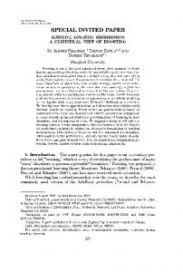
LOGISTIC REGRESSION AND GENERALISED LINEAR MODELS data("plasma", package = "HSAUR") layout(matrix(1:2, ncol = 2)) cdplot(ESR ~ fibrinogen, data = plasma) cdplot(ESR ~ globulin, data = plasma)
ESR > 20
4 R> R> R> R>
30
35
40
45
globulin
Conditional density plots of the erythrocyte sedimentation rate (ESR) given fibrinogen and globulin.
2.5 % 97.5 % 1.403209 54.515884
The confidence interval is very wide because there are few observations overall and very few where the ESR value is greater than 20. Nevertheless it seems likely that increased values of fibrinogen lead to a greater probability of an ESR value greater than 20. We can now fit a logistic regression model that includes both explanatory variables using the code R> plasma_glm_2 summary(plasma_glm_1) Call: glm(formula = ESR ~ fibrinogen, family = binomial(), data = plasma) Deviance Residuals: Min 1Q Median -0.9298 -0.5399 -0.4382
3Q -0.3356
Max 2.4794
Coefficients: Estimate Std. Error z value Pr(>|z|) (Intercept) -6.8451 2.7703 -2.471 0.0135 * fibrinogen 1.8271 0.9009 2.028 0.0425 * --Signif. codes: 0 '***' 0.001 '**' 0.01 '*' 0.05 '.' 0.1 ' ' 1 (Dispersion parameter for binomial family taken to be 1) Null deviance: 30.885 Residual deviance: 24.840 AIC: 28.84
on 31 on 30
degrees of freedom degrees of freedom
Number of Fisher Scoring iterations: 5
Figure 6.2
R output of the summary method for the logistic regression model fitted to the plasma data.
R> anova(plasma_glm_1, plasma_glm_2, test = "Chisq") Analysis of Deviance Table Model 1: Model 2: Resid. 1 2
ESR ~ fibrinogen ESR ~ fibrinogen + globulin Df Resid. Dev Df Deviance Pr(>Chi) 30 24.840 29 22.971 1 1.8692 0.1716
Nevertheless we shall use the predicted values from the second model and plot them against the values of both explanatory variables using a bubble plot to illustrate the use of the symbols function. The estimated conditional probability of a ESR value larger 20 for all observations can be computed, following formula (??), by R> prob summary(plasma_glm_2) Call: glm(formula = ESR ~ fibrinogen + globulin, family = binomial(), data = plasma) Deviance Residuals: Min 1Q Median -0.9683 -0.6122 -0.3458
3Q -0.2116
Max 2.2636
Coefficients: Estimate Std. Error z value Pr(>|z|) (Intercept) -12.7921 5.7963 -2.207 0.0273 * fibrinogen 1.9104 0.9710 1.967 0.0491 * globulin 0.1558 0.1195 1.303 0.1925 --Signif. codes: 0 '***' 0.001 '**' 0.01 '*' 0.05 '.' 0.1 ' ' 1 (Dispersion parameter for binomial family taken to be 1) Null deviance: 30.885 Residual deviance: 22.971 AIC: 28.971
on 31 on 29
degrees of freedom degrees of freedom
Number of Fisher Scoring iterations: 5
Figure 6.3
R output of the summary method for the logistic regression model fitted to the plasma data.
the two explanatory variables, sex and education. To fit a logistic regression model to such grouped data using the glm function we need to specify the number of agreements and disagreements as a two-column matrix on the left hand side of the model formula. We first fit a model that includes the two explanatory variables using the code R> data("womensrole", package = "HSAUR") R> fm1 womensrole_glm_1 role.fitted1 myplot symbols(plasma$fibrinogen, plasma$globulin, circles = prob, + add = TRUE)
●
●
30
●●
●
● ●
●
25
●
2
3
4
5
6
fibrinogen
Figure 6.4
+ + + + + + + + + +
Bubble plot of fitted values for a logistic regression model fitted to the ESR data.
xlab = "Education", ylim = c(0,1)) lines(womensrole$education[!f], role.fitted[!f], lty = 1) lines(womensrole$education[f], role.fitted[f], lty = 2) lgtxt |z|) (Intercept) 2.50937 0.18389 13.646 data("polyps", package = "HSAUR") R> polyps_glm_1 summary(womensrole_glm_2) Call: glm(formula = fm2, family = binomial(), data = womensrole) Deviance Residuals: Min 1Q -2.39097 -0.88062
Median 0.01532
3Q 0.72783
Max 2.45262
Coefficients: Estimate Std. Error z value Pr(>|z|) (Intercept) 2.09820 0.23550 8.910 < 2e-16 sexFemale 0.90474 0.36007 2.513 0.01198 education -0.23403 0.02019 -11.592 < 2e-16 sexFemale:education -0.08138 0.03109 -2.617 0.00886 --Signif. codes: 0 '***' 0.001 '**' 0.01 '*' 0.05 '.' 0.1
*** * *** ** ' ' 1
(Dispersion parameter for binomial family taken to be 1) Null deviance: 451.722 Residual deviance: 57.103 AIC: 203.16
on 40 on 37
degrees of freedom degrees of freedom
Number of Fisher Scoring iterations: 4
Figure 6.7
R output of the summary method for the logistic regression model fitted to the womensrole data.
We can deal with overdispersion by using a procedure known as quasilikelihood, which allows the estimation of model parameters without fully knowing the error distribution of the response variable. McCullagh and Nelder (1989) give full details of the quasi-likelihood approach. In many respects it simply allows for the estimation of φ from the data rather than defining it to be unity for the binomial and Poisson distributions. We can apply quasilikelihood estimation to the colonic polyps data using the following R code R> polyps_glm_2 summary(polyps_glm_2) Call: glm(formula = number ~ treat + age, family = quasipoisson(), data = polyps) Deviance Residuals: Min 1Q Median -4.2212 -3.0536 -0.1802
3Q 1.4459
Max 5.8301
Coefficients: Estimate Std. Error t value Pr(>|t|) (Intercept) 4.52902 0.48106 9.415 3.72e-08 *** treatdrug -1.35908 0.38533 -3.527 0.00259 ** age -0.03883 0.01951 -1.991 0.06284 . ---
1.0
ANALYSIS USING R 11 R> role.fitted2 myplot(role.fitted2)
0.6 0.4 0.0
0.2
Probability of agreeing
0.8
Fitted (Males) Fitted (Females)
0
5
10
15
20
Education
Figure 6.8
Fitted (from womensrole_glm_2) and observed probabilities of agreeing for the womensrole data.
Signif. codes:
0 '***' 0.001 '**' 0.01 '*' 0.05 '.' 0.1 ' ' 1
(Dispersion parameter for quasipoisson family taken to be 10.72805) Null deviance: 378.66 Residual deviance: 179.54 AIC: NA
on 19 on 17
degrees of freedom degrees of freedom
Number of Fisher Scoring iterations: 5
The regression coefficients for both explanatory variables remain significant but their estimated standard errors are now much greater than the values given in Figure 6.10. A possible reason for overdispersion in these data is that
12 LOGISTIC REGRESSION AND GENERALISED LINEAR MODELS R> res plot(predict(womensrole_glm_2), res, + xlab="Fitted values", ylab = "Residuals", + ylim = max(abs(res)) * c(-1,1)) R> abline(h = 0, lty = 2)
●
2
●
● ● ● ●
1
●
●
●
●
●
●
●
● ●
●
0
Residuals
●
● ●
●
●
● ●
●
●
● ●
● ● ●
−1
●
●
● ●
● ●
●
●
●
−2
● ● ●
−3
−2
−1
0
1
2
3
Fitted values
Figure 6.9
Plot of deviance residuals from logistic regression model fitted to the womensrole data.
polyps do not occur independently of one another, but instead may ‘cluster’ together.
ANALYSIS USING R
13
R> summary(polyps_glm_1) Call: glm(formula = number ~ treat + age, family = poisson(), data = polyps) Deviance Residuals: Min 1Q Median -4.2212 -3.0536 -0.1802
3Q 1.4459
Max 5.8301
Coefficients: Estimate Std. Error z value Pr(>|z|) (Intercept) 4.529024 0.146872 30.84 < 2e-16 *** treatdrug -1.359083 0.117643 -11.55 < 2e-16 *** age -0.038830 0.005955 -6.52 7.02e-11 *** --Signif. codes: 0 '***' 0.001 '**' 0.01 '*' 0.05 '.' 0.1 ' ' 1 (Dispersion parameter for poisson family taken to be 1) Null deviance: 378.66 Residual deviance: 179.54 AIC: 273.88
on 19 on 17
degrees of freedom degrees of freedom
Number of Fisher Scoring iterations: 5
Figure 6.10
R output of the summary method for the Poisson regression model fitted to the polyps data.
Bibliography McCullagh, P. and Nelder, J. A. (1989), Generalized Linear Models, London, UK: Chapman & Hall/CRC.