Beyond the Standard Model B-parameters with improved staggered ...

arXiv:1310.7372v1 [hep-lat] 28 Oct 2013

Beyond the Standard Model B-parameters with improved staggered fermions in N f = 2 + 1 QCD

Taegil Bae, Yong-Chull Jang, Hwancheol Jeong, Jangho Kim, Jongjeong Kim, Kwangwoo Kim, Seonghee Kim, Weonjong Lee, Jaehoon Leem Lattice Gauge Theory Research Center, CTP, and FPRD, Department of Physics and Astronomy, Seoul National University, Seoul, 151-747, South Korea E-mail: [email protected]

Hyung-Jin Kim, Chulwoo Jung Physics Department, Brookhaven National Laboratory, Upton, NY11973, USA E-mail: [email protected]

Stephen R. Sharpe Physics Department, University of Washington, Seattle, WA 98195-1560, USA E-mail: [email protected]

Boram Yoon∗ Los Alamos National Laboratory, MS B283, P.O. Box 1663, Los Alamos, NM 87545, USA E-mail: [email protected]

SWME Collaboration We calculate the kaon mixing B-parameters for operators arising generically in theories of physics beyond the standard model. We use HYP-smeared improved staggered fermions on the N f = 2 + 1 MILC asqtad lattices. Operator matching is done perturbatively at one-loop order. Chiral extrapolations are done using “golden combinations” in which one-loop chiral logarithms are absent. For the combined sea-quark mass and continuum extrapolation, we use three lattice spacings: a ≈ 0.045, 0.06 and 0.09 fm. Our results have a total error of 5-6%, which is dominated by the systematic error from matching and continuum extrapolation. For two of the BSM B-parameters, we agree with results obtained using domain-wall and twisted-mass dynamical fermions, but we disagree by (4 − 5)σ for the other two.

The 31st International Symposium on Lattice Field Theory - Lattice 2013 July 29 – August 3, 2013 Mainz, Germany ∗ Speaker.

c Copyright owned by the author(s) under the terms of the Creative Commons Attribution-NonCommercial-ShareAlike Licence.

http://pos.sissa.it/

BSM B-parameters with Staggered Fermions

Boram Yoon

1. Introduction Kaon mixing, and in particular the CP-violating component εK , can provide powerful constraints on theories of physics beyond the standard model (BSM). BSM theories lead to contributions to the mixing amplitude which add to that from the standard model (SM). Given that we now know the SM contributions to εK quite accurately, there is little room for BSM additions. In order to determine the constraints on the parameters of BSM models, one needs to know the matrix elements of the local four-fermion ∆S = 2 operators that arise when new, BSM heavy particles are integrated out. It turns out that, in addition to the operator appearing in the shortdistance component of the SM contribution (which has a “left-left” Dirac structure and whose matrix element is parametrized by BK ), BSM theories lead to four other operators. Here we present our results for the matrix elements of all five operators, and compare with those of other recent calculations [1, 2]. More details of our results are given in Ref. [3].

2. Methodology and Results We adopt the operator basis used in Ref. [4], Q1 = [s¯a γµ (1 − γ5 )d a ][s¯b γµ (1 − γ5 )d b ] , Q2 = [s¯a (1 − γ5 )d a ][s¯b (1 − γ5 )d b ] , Q3 = [s¯a σµν (1 − γ5 )d a ][s¯b σµν (1 − γ5 )d b ] ,

(2.1)

Q4 = [s¯ (1 − γ5 )d ][s¯ (1 + γ5 )d ] , a

a

b

b

Q5 = [s¯a γµ (1 − γ5 )d a ][s¯b γµ (1 + γ5 )d b ] , where a, b are color indices and σµν = [γµ , γν ]/2. Q1 is the SM operator while Q2−5 are the BSM operators. Matrix elements of the latter are parametrized as Bi ( µ ) =

hK 0 |Qi (µ )|K0 i Ni hK 0 |sγ5 d(µ )|0ih0|s¯γ5 d(µ )|K0 i

(2.2)

(N2 , N3 , N4 , N5 ) = (5/3, 4, −2, 4/3) . The basis (2.1) is that in which the the two-loop anomalous dimensions (which we use for renormalization group running) are known [4]. It differs from the “SUSY” basis of Ref. [5] (which has been used in previous lattice calculations of the BSM matrix elements), although the two bases are simply related, as discussed below. Table 1 shows the lattices used in this work. They are generated using N f = 2 + 1 flavors of asqtad staggered quarks [6]. For valence quarks, we use HYP-smeared staggered fermions [7]. The calculation of the BSM B-parameters follows closely the methodology used in our BK calculation [8, 9]. The lattice operators are matched, at one-loop order, to continuum operators defined in the renormalization scheme of Ref. [4]. This scheme differs slightly from that used in the continuum-lattice matching calculation of Ref. [10], requiring an additional (continuum) matching factor which we have calculated. The matching on each lattice is done at a renormalization scale µ = 1/a, with results subsequently run to a common final scale using the continuum two-loop anomalous dimensions. 2

BSM B-parameters with Staggered Fermions

Boram Yoon

Table 1: MILC lattices used in this calculation. Here “ens” is the number of gauge configurations, “meas” is the number of measurements per configuration, and ID identifies the ensemble.

a (fm) 0.09 0.09 0.09 0.09 0.09 0.06 0.06 0.06 0.06 0.045

amℓ / ams 0.0062 / 0.031 0.0093 / 0.031 0.0031 / 0.031 0.0124 / 0.031 0.00465 / 0.031 0.0036 / 0.018 0.0072 / 0.018 0.0025 / 0.018 0.0054 / 0.018 0.0028 / 0.014

size 283 × 96 283 × 96 403 × 96 283 × 96 323 × 96 483 × 144 483 × 144 563 × 144 483 × 144 643 × 192

ens × meas 995 × 9 949 × 9 959 × 9 1995 × 9 651 × 9 749 × 9 593 × 9 799 × 9 582 × 9 747 × 1

ID F1 F2 F3 F4 F5 S1 S2 S3 S4 U1

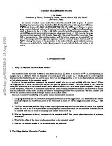
n (with n = 1 − 10), where mx We use ten different valence quark masses, amx,y = ams × 10 and my are the valence d and s quark masses, respectively, while ms (given in Table 1) lies close to the physical strange quark mass. Thus our valence pion masses run down almost to 200 MeV. Results are extrapolated to physical light-quark masses using SU(2) staggered chiral perturbation theory (SChPT), taking the lightest four quark masses for mx and the heaviest three for my . Thus we remain in the regime, mx ≪ my ∼ ms , where we expect SU(2) ChPT to be applicable. As an example of the quality of our data, we show, in Fig. 1, the plateaus that we find for B2 on the three lattice spacings. This is for our most kaon-like choice of valence quark masses. We use U(1) noise sources to create kaons with a fixed separation, and place the lattice operators between them. From plots such as these, as well as those for kaon correlators, we determine how far from the sources we must work to avoid excited-state contamination. We then fit to a constant. Generalizing a proposal of Ref. [11], Ref. [12] suggested that chiral extrapolations of BSM B-parameters would be simpler if one uses the following “golden combinations”:

G23 =

B2 , B3

G45 =

B4 , B5

G24 = B2 · B4 ,

G21 =

B2 . BK

(2.3)

This is because the leading chiral logarithms, which appear at next-to-leading order (NLO) in ChPT, cancel in these quantities (if one uses SU(2) ChPT). This observation is particularly important for staggered fermions, since chiral logarithms introduce taste-breaking effects which normally have to be corrected for. Hence, we perform the chiral and continuum extrapolations using the golden combinations, as well as BK , and obtain our final results by inverting Eq. (2.3). We obtain consistent results by directly extrapolating the B-parameters themselves using the SU(2) SChPT forms of Ref. [12], following the analysis method previously followed for BK [8, 9]. To extrapolate in mx , we fit the golden combinations to Gi (X-fit) = c1 + c2 X + c3 X 2 + c4 X 2 ln2 X + c5 X 2 ln X + c6 X 3 , 3

(2.4)

BSM B-parameters with Staggered Fermions

Boram Yoon

Figure 1: B2 (µ = 1/a) as a function of T , the distance between the left-hand kaon source and the operator. (Blue) diamonds, (purple) octagons and (brown) squares are from the F1, S1, and U1 ensembles, respectively, with (mx , my ) = (ms /10, ms ).

where X ≡ XP /Λ2χ with XP = Mπ2:xx¯ , and Λχ = 1 GeV, and generic NNLO continuum chiral logarithms are included. We call this the X-fit. To fit our four data points to this form, we constrain the coefficients c4−6 with Bayesian priors: ci = 0 ± 1. Systematic errors in X-fits are estimated by doubling the widths of these priors, and by comparing to the results of the eigenmode shift method [13]. The X-fits for BK do involve NLO chiral logarithms, and we follow the same procedure as in Refs. [8, 9]. The extrapolation in the valence strange mass my is done using a linear function of YP = Mπ2:yy¯ , with a quadratic fit used to estimate a systematic error. We call this the Y-fit. In Fig. 2, we show Xand Y-fits for G23 , illustrating the mild dependence on the valence quark masses. After these valence chiral extrapolations, we have, for each ensemble, results for the the Gi (and BK ) at scale µ = 1/a. We next evolve these to a common scale, either 2 GeV or 3 GeV, using the two-loop anomalous dimensions of Ref. [4]. These results can then be extrapolated to the continuum and to physical sea-quark masses (with the dependence on the latter being analytic at NLO). We do a simultaneous extrapolation using f1 = d1 + d2 (aΛQ )2 + d3 LP /Λ2χ + d4 SP /Λ2χ ,

(2.5)

where LP and SP are squared masses of taste-ξ5 pions composed of two light sea quarks and two strange sea quarks, respectively. Discretization errors are scaled with ΛQ = 300 MeV, so that for a typical discretization error one would have d2 ∼ O(1). However, we find that d2 ∼ 2 − 7 for the golden combinations, indicating enhanced lattice artifacts. The artifacts in BK are much smaller. These results are illustrated in Fig. 3. The extrapolation fits have χ 2 /dof in the range 1.6 − 2.7. 4

BSM B-parameters with Staggered Fermions

Boram Yoon

1.394

1.394 1.393

1.393 G23

G23

1.392 1.392

1.391 1.39

1.391 1.389 1.39

1.388 0

0.05

0.1 XP (GeV2)

0.15

0.2

0.3

(a) X-fit

0.35

0.4 YP (GeV2)

0.45

0.5

(b) Y-fit

Figure 2: (a) X-fit and (b) Y-fit of G23 (µ = 1/a) on F1 ensemble. In the X-fit, my is fixed at amy = 0.03. The red diamond represents the extrapolated physical point in both plots. 1.44

Fine Superfine Ultrafine

0.54

G23 (2GeV)

BK (2GeV)

0.56

0.52

0.5

1.42

1.4 Fine Superfine Ultrafine

1.38 0

0.1

0.2

0

0.1

LP (GeV2)

0.2

LP (GeV2)

(a) BK

(b) G23

Figure 3: Examples of simultaneous sea-quark mass and continuum extrapolations. Red circles denote extrapolated results.

To estimate the systematic uncertainty in the continuum extrapolation, we compare the results of fitting to Eq. (2.5) with those obtained using the following fitting function, which includes higher order terms in a2 and αs [which here means αsMS (1/a)]: f2 = f1 + d5 (aΛQ )2 αs + d6 αs2 + d7 (aΛQ )4 .

(2.6)

The difference, ∆ f12 = | f1 − f2 |, is about 5%, and is comparable with our estimate of the systematic error coming from the one-loop matching, which we estimate by αs2 (U1) = 4.4%. Since Eq. (2.6) includes terms of αs2 , it also captures the systematic error from using one-loop perturbative matching. Hence, we quote the larger of ∆ f12 and αs2 (U1) in our final error budget for the matching/continuum extrapolation error. In Table 2, we show our final results for the B-parameters evaluated at µ = 2 GeV and 3 GeV. Total errors are 5 − 6%, and are dominated the systematic errors, as can be seen from the error budget given in Table 3. Further details concerning error estimates are explained in Ref. [3]. Overall, we see that the matching/continuum extrapolation dominates. 5

BSM B-parameters with Staggered Fermions

Boram Yoon

Table 2: Results for the Bi at µ = 2 GeV and 3 GeV.

BK B2 B3 B4 B5

µ = 2 GeV 0.537 (7)(24) 0.620 (4)(31) 0.433 (3)(19) 1.081 (6)(48) 0.853 (6)(49)

µ = 3 GeV 0.519 (7)(23) 0.549 (3)(28) 0.390 (2)(17) 1.033 (6)(46) 0.855 (6)(43)

Table 3: Error budget (in percent) for the Bi (2 GeV).

source of error ( statistics )

matching cont-extrap. X-fit (F1) Y-fit (F1) finite volume r1 = 0.3117(22) fm fπ = 132 vs. 124 MeV (F1)

BK 1.37

B2 0.64

B3 0.63

B4 0.60

B5 0.66

4.40

4.95

4.40

4.40

5.69

0.10 0.62 0.50 0.34 0.46

0.10 0.12 0.50 0.18 0.46

0.10 0.19 0.50 0.17 0.46

0.12 0.22 0.50 0.05 0.46

0.12 0.16 0.50 0.02 0.46

3. Comparisons and Outlook As noted above, there are two previous calculations of the BSM B-parameters using dynamical quarks: one using N f = 2 + 1 flavors of domain-wall fermions at a single lattice spacing [1], the other using N f = 2 flavors of twisted-mass fermions at three lattice spacings [2]. The results from these two calculations are consistent. We pick those of Ref. [1] for a detailed comparison with our results, since then both calculations use the same number of dynamical flavors. We begin by noting that the results for BK in all three calculations are consistent (within the small errors). For the BSM B-parameters, Ref. [1] finds, at µ = 3 GeV, that BSUSY 2−5 = 0.43(5), 0.75(9), 0.69(7) and 0.47(6), respectively. These are calculated in the SUSY basis, in which BSUSY = (5B2 − 3B3 )/2, while the other three B-parameters are the same. Our results convert 3 = 0.79(3). Using this, and Table 2, we see that, while B2 and B3 are (at µ = 3 GeV) to BSUSY 3 consistent, B4 and B5 are not. Our results are 1.5 and 1.8 times larger, respectively, a difference of 4 − 5σ . At the present time, we do not know the origin of this difference. We have ruled out the simplest possibilities, such as using incorrect continuum anomalous dimensions, by various cross checks with results in the literature. It thus seems that systematic errors in one or both calculations are being underestimated, the most likely culprit being the estimate of the truncation error in matching. This enters at the two-loop level in both calculations, since both are ultimately connected to a 6

BSM B-parameters with Staggered Fermions

Boram Yoon

continuum scheme by one-loop matching. We think it is important to resolve this disagreement, not only because the matrix elements are wanted for phenomenology, but also because it may impact the reliability of other calculations. One way to proceed is for all calculations to use a common (S)MOM scheme and non-perturbative renormalization and running. This avoids the matching to the continuum. We are working in this direction. Another idea is for the other calculations to do the chiral extrapolations using the golden combinations described above.

Acknowledgments We thank Claude Bernard for providing unpublished information. W. Lee is supported by the Creative Research Initiatives program (2013-003454) of the NRF grant funded by the Korean government (MSIP). C. Jung and S. Sharpe are supported in part by the US DOE through contract DE-AC02-98CH10886 and grant DE-FG02-96ER40956, respectively. Computations for this work were carried out in part on the QCDOC computer of the USQCD Collaboration, funded by the Office of Science of the US DOE. W. Lee acknowledges support from the KISTI supercomputing center through the strategic support program [No. KSC-2012-G3-08].

References [1] RBC/UKQCD Collaboration, P. Boyle, N. Garron, and R. Hudspith Phys.Rev. D86 (2012) 054028, [arXiv:1206.5737]. [2] ETM Collaboration, V. Bertone et al. JHEP 1303 (2013) 089, [arXiv:1207.1287]. [3] SWME Collaboration, T. Bae et al. arXiv:1309.2040. [4] A. J. Buras, M. Misiak, and J. Urban Nucl.Phys. B586 (2000) 397–426, [hep-ph/0005183]. [5] F. Gabbiani, E. Gabrielli, A. Masiero, and L. Silvestrini Nucl.Phys. B477 (1996) 321–352, [hep-ph/9604387]. [6] A. Bazavov, D. Toussaint, C. Bernard, J. Laiho, C. DeTar, et al. Rev.Mod.Phys. 82 (2010) 1349–1417, [arXiv:0903.3598]. [7] A. Hasenfratz and F. Knechtli Phys.Rev. D64 (2001) 034504, [hep-lat/0103029]. [8] T. Bae, Y.-C. Jang, C. Jung, H.-J. Kim, J. Kim, et al. Phys.Rev. D82 (2010) 114509, [1008.5179]. [9] T. Bae et al. Phys.Rev.Lett. 109 (2012) 041601, [1111.5698]. [10] J. Kim, W. Lee, and S. R. Sharpe Phys.Rev. D83 (2011) 094503, [arXiv:1102.1774]. [11] D. Becirevic and G. Villadoro Phys.Rev. D70 (2004) 094036, [hep-lat/0408029]. [12] J. A. Bailey, H.-J. Kim, W. Lee, and S. R. Sharpe Phys.Rev. D85 (2012) 074507, [1202.1570]. [13] B. Yoon, Y.-C. Jang, C. Jung, and W. Lee J.Korean Phys.Soc. 63 (2013) 145–162, [arXiv:1101.2248].

7