Bias reduction in skewed binary classification with Bayesian neural networks. P.J.G. Lisboa*, A. Vellido, H. Wong. School of Computing and Mathematical ...
Neural Networks PERGAMON
Neural Networks 13 (2000) 407–410 www.elsevier.com/locate/neunet
Neural Networks Letter
Bias reduction in skewed binary classification with Bayesian neural networks P.J.G. Lisboa*, A. Vellido, H. Wong School of Computing and Mathematical Sciences, Liverpool John Moores University, Liverpool L3 3AF, UK Received 12 February 2000; accepted 17 February 2000
Abstract The Bayesian evidence framework has become a standard of good practice for neural network estimation of class conditional probabilities. In this approach the conditional probability is marginalised over the distribution of network weights, which is usually approximated by an analytical expression that moderates the network output towards the midrange. In this paper, it is shown that the network calibration is considerably improved by marginalising to the prior distribution. Moreover, marginalisation to the midrange can seriously bias the estimates of the conditional probabilities calculated from the evidence framework. This is especially the case in the modelling of censored data. 䉷 2000 Elsevier Science Ltd. All rights reserved. Keywords: Calibration; Marginalisation; Bayesian neural networks; Bias
1. Introduction The Bayesian framework for neural networks (MacKay, 1992) is widely used as a practical methodology for binary classification. Inherent in this framework is the prediction of distributions for the network weights, such that the estimation of the conditional probability of class membership is a marginalisation over the probability density for the weights yg
x
Z y
aP
a兩x; D da;
1
where y
a
w; x is the actual network output, P
a兩x; D the posterior distribution of the network activation, and yg
x ⬃ P
Class兩x the conditional. In general, this integral is not analytic due to the non-linearities in the output response y
x g
a
x;
g
a 1=
1 ⫹ exp
⫺a;
therefore it is approximated to ! a
x yg
x ⬇ g p ; 1 ⫹ p s2
x=8
2
3
where a(x) represents the output node activation in response to input pattern x, and s2
x is the associated variance for the weights. Whether or not this approximation is employed, the effect of uncertainty in the weights remains the same, * Corresponding author.
namely to moderate the network predictions towards the midrange. However, the presence of uncertainty should moderate the conditional towards the best unconditional estimate, which is the class prior. This paper shows that marginalising to the prior specifies a preferred cost function weighting scheme, which has the effect of substantially reducing the bias in the estimates of the class conditional obtained from the Bayesian neural networks.
2. Methodology It is proposed that the estimate of the conditional using the evidence approximation should be obtained in two stages. First, by training the network to equal priors, then, using the Bayes theorem to refer the estimates of the conditional back to the true priors. The prior distribution seen by the model can be equalised by weighting the cost function (Lowe & Webb, 1991) ! X 1 LL ⫺ ⫹
1 ⫺ tlog
1 ⫺ y
tlog
y 2P
Class samples ×
1 2
1 ⫺ P
Class
!!
4
updating the gradient and the Hessian calculations in the
0893-6080/00/$ - see front matter 䉷 2000 Elsevier Science Ltd. All rights reserved. PII: S0893-608 0(00)00022-8
408
P.J.G. Lisboa et al. / Neural Networks 13 (2000) 407–410
Fig. 1. Direct modelling of the skewed data: calibration of the original network outputs in the prediction of propensity to purchase on the web (dashed line) and following marginalisation to the midrange (solid line). A measure of the calibration error is the RMS distance for the calibration line to the diagonal, which is 0.034 before marginalisation, and becomes 0.042 afterwards.
same way. The network estimates of the conditional are then ! Z ~ a
x ~ ~ xP
w兩x2 w ⬇ g p
5 y~g
x y
w; 1 ⫹ p s~2
x=8 where the tilde denotes equal priors. These estimates are sometimes obtained by sub-sampling the data, or even by augmenting the data using noisy re-samples (Lee, 1999). Our approach utilises all of the actual data and avoids the need for further artificial data. The correct estimate of the conditional is readily obtained from the Bayes theorem in the usual way (Tarassenko, 1998) P
Class兩x ⬇ yg
x
y~g
xP
Class ; y~g
xP
Class ⫹
1 ⫺ y~g
x
1 ⫺ P
Class
6
which has the required property that yg
x ! P
Class when y~g
x ! 0:5: This transformation corresponds to a linear shift of the log–odds ratio of the balanced distribution, which is the network activation, by an amount given by the log–odds of the class priors, since ! ! y~g
x yg
x log log
1 ⫺ yg
x
1 ⫺ y~g
x � � P
Class :
7 ⫹ log
1 ⫺ P
Class Therefore, the above procedure can be interpreted as estimating the distribution of the network output activations
Fig. 2. Compensation for uneven priors: calibration of the original network outputs weighting the cost function towards balanced data (long dash), and following referral to the assumed class prior (dashed line) and marginalisation (solid line). The calibration accuracies before and after marginalisation are now 0.045 and 0.032.
near the region of highest slope for the output response, rather than on the tail of the sigmoid.
3. Marginalisation results The effect on the network calibration, of marginalising to an appropriate class prior, is illustrated in this section with two contrasting examples. We consider, first, a standard predictive application of propensity to buy on the internet. The second example is more demanding of calibration accuracy, and concerns survival modelling. In each case, the data are split into roughly equal training and test sets, and the class prior is approximated to the prevalence observed in the training data. A public domain survey of the attitudes of web users to electronic commerce forms the basis for modelling propensity to buy on-line, as a mechanism to identify the most predictive variables for later use in a segmentation study (Vellido, Lisboa & Meehan, 1999). Figs. 1 and 2 show the calibration curves which result, first from the standard Bayesian–ARD model, trained directly on the skewed data, then using the proposed marginalisation to the empirical class prior with an identical network structure. The mean and standard deviation of the test results from 20 networks trained on 895 purchasers and 194 nonpurchasers are shown, and tested on as many out-of-sample records. The calibration accuracy is quantified by measuring the RMS error between the empirical calibration and the ideal line, digitised into intervals indexed
P.J.G. Lisboa et al. / Neural Networks 13 (2000) 407–410
409
ROC curve measures the ability of the classifier to rank samples correctly from the two classes, but does not directly test its calibration accuracy. Good calibration is essential where the network outputs are multiplied in sequence, as when dealing with censorship. Censored data are common in survival modelling when the endpoint of an individual follow-up is not the event of interest. In the modelling of survival following surgery for breast cancer, for instance, censorship applies to patients lost to follow-up through any cause other than death from breast cancer, and also to patients who survive beyond the end of the timeframe for the study. The reasons for censorship range from moving away from the geographical area of follow-up to death by an unrelated cause. Either way, the outcome for that patient is known only for part of the intended follow-up period, therefore it is entered into the log-likelihood cost function (Eq. (4)) only for the time intervals where the patient is observed with a target of 0 when the patient is observed alive, and 1 for the time interval during which death from breast cancer occurred. Consequently, the number of targets entered is different for different patients, and not all patients ever include a target value of unity. In survival modelling the quantity of interest is the hazard rate, which denotes the probability for the occurrence of the event of interest within a particular time interval h
ti ; x P
ti⫺1 ⬍ t ⬍ ti 兩x ⬃ yg
ti ; x:
9
Under the assumption of the conditional independence of successive time intervals, the survival curve follows by successive multiplication of the hazard rates
Fig. 3. Predicted discrete time hazard rates for breast cancer patients following surgery. Notice that the scale of the hazard estimates for the balanced ~ distribution, y
x; in (a) is very much larger than the final estimates, y
x, in (b). The effect of marginalisation shows in the crossing of the hazard estimates in each case, around the mid-range and at the mean hazard of 0.0032.
by i AccCAL sqrt
"no: output intervals X
#
cal
i ⫺ y
i p
y
i : 2
8
i1
It is clear from the numerical results quoted in the figure captions that the standard Bayesian neural network procedure introduces the calibration bias as a result of a systematic shift of the calibration curve on either side of the midrange. This effect becomes important for skewed binary classification since the distribution of network outputs is not symmetrical about the midpoint. The Receiver Operating Characteristic (ROC) curves for both of these methods are very similar, with sensitivity and specificity values for a sweep of classification thresholds simply sliding along a common envelope. This arises because the area under the
S
tk ; x
k Y
h
ti ; x:
10
i1
An adaptation of the standard MLP model by optimising to a partial log-likelihood cost function with time as a covariate, alongside the static patient attributes, is called the Partial Logistic Artificial Neural Network (Biganzoli, Boracchi, Mariani & Marubini, 1998). The standard evidence framework was applied to the PLANN model (Wong, Harris, Lisboa, Kirby & Swindell, 1999), and compared with marginalisation to the average hazard rate, using 917 patient records. The hazard rates and survival were estimated by 5-fold cross validation, with the results shown in Figs. 3 and 4. As the resolution of the time intervals increases the frequency of events in each time interval reduces, resulting in a very skewed distribution for the discrete time hazard. The simplest way to compensate for this in a Bayesian neural network is to marginalise to the empirical mean hazard rate. The class prevalence in each time interval is measured from the training samples in the same way as before, by taking the ratio of unity targets to the total number of targets, including those for censored patients, which is then averaged over the time intervals.
410
P.J.G. Lisboa et al. / Neural Networks 13 (2000) 407–410
systematic bias. The low survival of the highest risk cohort has its survival slightly over estimated, as a direct result of the marginalisation towards the group mean of the hazard. A further improvement to the prediction of survival for that group is readily obtained by modelling them separately from the rest, since they represent a high risk subgroup within what was initially thought to be a low risk cohort of patients. A corollary to these results is that, in mixed populations, the neural network derived estimates of the class conditional will be necessarily biased towards the overall class mean. In some applications, the residual of the calibration may act as a diagnostic test to help break-up the data into separate cohorts with difference characteristic priors. 4. Conclusion Marginalisation to the class prior in Bayesian neural networks trained with unequal class prevalences minimises the risk of biasing the calibration, which results from defaulting towards the midrange of the network output. In survival modelling, this procedure is essential to avoid introducing a substantial bias into the model predictions but, in all binary classification problems with skewed data, the default marginalisation introduces a systematic shift away from correct calibration. Moreover, the proposed application of the evidence framework avoids the need to artificially change the sampling procedure in order to equalise the priors, and indicates a preferred weighting scheme for the log-likelihood cost function, which applies uniformly for both observed and censored data. Fig. 4. (a) Predicted, and (b) the observed survival for patients grouped by a prognostic index (Biganzoli et al., 1998) derived from the log–odds ratio, and aggregated using the log-rank test. The lower four curves in (a) result from marginalising the hazard rates to 0.5 in each of the 72 time intervals, and the upper curves from marginalising to the overall mean hazard. It is clear that the default Bayesian neural network procedure, in this case, introduces an unacceptable level of bias in the predictions. The effect of marginalising to the average survival curve is apparent in (a), where the higher risk group has its survival estimates biased upwards towards the group mean. This group can be modelled separately to bring the predicted survival inside the one standard deviation bands in the Kaplan–Meier curves in (b).
Marginalising the hazard to 0.5 now has the effect of uniformly raising the hazard rates away from their true value, introducing an unacceptable level of bias that is evident from the survival curves. This effect is compounded by the sequential multiplication of hazards. In contrast, the proposed procedure stabilises the network output, permitting correction for uncertainty using the evidence approximation and the resulting survival curves have no apparent
References Biganzoli, E., Boracchi, P., Mariani, L., & Marubini, E. (1998). Feedforward neural networks for the analysis of censored survival data: a partial logistic regression approach. Statistics in Medicine, 17, 1169– 1186. Lee, S. S. (1999). Regularization in skewed binary classification. Computational Statistics, 14 (2), 277–292. Lowe, D., & Webb, A. R. (1991). Optimized feature extraction and the Bayes decision in feed-forward classifier networks. Institute of Electrical and Electronics Engineers-Pattern Analysis and Machine Intelligence, 13 (4), 355–364. MacKay, D. J. C. (1992). The evidence framework applied to classification networks. Neural Computation, 4 (5), 720–736. Tarassenko, L. (1998). A guide to neural computing applications. London: Wiley. Vellido, A., Lisboa, P. J. G., & Meehan, K. (1999). Segmentation of the online shopping market using neural networks. Expert Systems with Applications, 17, 303–314. Wong, H., Harris, P., Lisboa, P. J. G., Kirby, S. P. J., & Swindell, R. (1999). Dealing with Censorship in Neural Network Models. International Joint Conference on Neural Networks, Washington, DC, Paper No. 388.