Biclustering of Expression Microarray Data Using Affinity Propagation

Biclustering of Expression Microarray Data Using Affinity Propagation Alessandro Farinelli, Matteo Denitto, and Manuele Bicego University of Verona, Department of Computer Science, Verona, Italy

Abstract. Biclustering, namely simultaneous clustering of genes and samples, represents a challenging and important research line in the expression microarray data analysis. In this paper, we investigate the use of Affinity Propagation, a popular clustering method, to perform biclustering. Specifically, we cast Affinity Propagation into the Couple Two Way Clustering scheme, which allows to use a clustering technique to perform biclustering. We extend the CTWC approach, adapting it to Affinity Propagation, by introducing a stability criterion and by devising an approach to automatically assemble couples of stable clusters into biclusters. Empirical results, obtained in a synthetic benchmark for biclustering, show that our approach is extremely competitive with respect to the state of the art, achieving an accuracy of 91% in the worst case performance and 100% accuracy for all tested noise levels in the best case.

1

Introduction

The recent wide employment of microarray tools in molecular biology and genetics have produced an enormous amount of data, which has to be processed to infer knowledge. Due to the dimension and complexity of those data, automatic tools coming from the Pattern Recognition research area have been successfully employed. Among others, clear examples are tools aiding the microarray probe design, the image processing-based techniques for the quantification of the spots (segmentation spot/background, grid matching, noise suppression [6]) and methodologies for classification or clustering [18,24,25,8]. In this paper we focus on this last class of problems and in particular on the clustering issue. Within this context, a recent trend is represented by the study and development of biclustering methodologies, namely techniques able to simultaneously group genes and samples; a bicluster may be defined as a subset of genes that show similar activity patterns under a specific subset of samples [20]. This kind of analysis may have a clear biological impact in the microarray scenario, where a bicluster may be associated to a biological process that is active only in some samples and may involve only a subset of genes. Different approaches to biclustering expression microarray data have been presented in the literature in the past, each one characterized by different features, like computational complexity, effectiveness, interpretability, optimization criterion and others (for a review see [20,22]). M. Loog et al. (Eds.): PRIB 2011, LNBI 7036, pp. 13–24, 2011. c Springer-Verlag Berlin Heidelberg 2011 

14

A. Farinelli, M. Denitto, and M. Bicego

It is worth noticing that, in many cases, successful methodologies have been obtained by adapting and tailoring advanced techniques developed in other fields of the Pattern Recognition research area. One clear example is represented by the topic models [14,5], initially designed for text mining and computer vision applications, and recently successfully applied in the microarray context [23,3,2]. Clearly, the peculiar context may lead to substantial changes in the model so to improve results [21]. This paper follows this promising direction, preliminary investigating the capabilities, in the expression microarray biclustering context, of a recent and powerful clustering technique, called Affinity Propagation (AP [10]). This technique is based on the idea of iteratively exchanging messages between data points until a proper set of representatives (called exemplars) are found. Such exemplars identify clusters (which are all points represented by a given exemplar). The efficacy of this algorithm (in terms of clustering accuracy) and its efficiency (due to its really fast learning algorithm) have been shown in many different application scenarios, including image analysis, gene detection and document analysis [10]. Moreover, AP seems to be a promising approach for the microarray scenario for two main reasons: first, AP does not need to know the number of clusters beforehand and in a microarray clustering problem it is often difficult to estimate a priori the number of groups, especially for the gene part; second, and more important, it is known that under some assumptions (e.g. sparse input data) this technique is very efficient for large scale problems such as microarray data which involves thousands of genes. Actually, in recent years some papers appeared in the literature with the aim of studying the application of this algorithm in the expression microarray field, in its basic version or in some more tailored ones [1,19,16,7]. Nevertheless, all these papers deal with the clustering problem, whereas the biclustering problem has not been addressed yet. In this paper, we propose an approach to use AP for biclustering based on a biclustering scheme called Coupled Two-Way Clustering (CTWC) [11], which iteratively performs samples and genes clustering using the supeparamagnetic clustering (SPC) algorithm, maintaining only clusters that satisfies a stability criterion (directly provided by the SPC clustering approach). In its original formulation CTWC does not provide an explicit representation of the obtained biclusters (which remain implicitly defined). Nevertheless, an automatic mechanism able to explicitly list the components of a bicluster is crucial for validation purposes (to the best of our knowledge, no biological validation tools deal with implicit or probabilistic memberships). To this end, in this paper we also proposed an automatic reassembling strategy, which may in principle be applied also to the original approach proposed in [11]. In more details this paper makes the following contribution to the state of the art: – Proposes the use of AP for biclustering. We cast AP into the CTWC biclustering scheme and propose a different stability criterion inspired from the bootstrapping, which is more general than the stability criterion used by CTWC and is well suited for the AP approach.

Biclustering of Expression Microarray Data Using Affinity Propagation

15

– Extends CTWC by devising an automatic reassembling strategy for the biclusters. The strategy takes as input the clusters obtained on rows and columns and returns only the couples of clusters that forms a bicluster in the input data. – Empirically tests the biclustering approach on a literature benchmark, using the synthetic data and protocols described in [22]. While a biological validation is clearly important to assess the practical significance of the approach, a synthetic validation permits to quantitatively compare the approach to other state of the art methods. In our experimental evaluation, we show that the proposed approach is very competitive with the literature, encouraging further investigations on the use of AP clustering algorithm in the microarray biclustering scenario. The remainder of the paper is organized as follows: Sect. 2 will introduce the Affinity Propagation clustering algorithm, whereas the proposed biclustering scheme is presented in Sect. 3. The experimental evaluation is detailed in Sect. 4; finally, in Sect. 5 conclusions are drawn and future perspectives are envisaged.

2

Background: Affinity Propagation

Affinity Propagation (AP) is a well known clustering technique recently proposed by Frey and Dueck [10] and successfully used in many different clustering contexts. The main idea behind AP is to perform clustering by finding a set of exemplar points that best represent the whole data set. This is carried out by viewing the input data as a network where each data point is a node, and selecting the exemplars by iteratively passing messages among the nodes. Messages convey the affinity that each point has for choosing another data point as its exemplar and the process stops when good exemplars emerge or after a predefined number of iterations. In more details, AP takes as input a similarity matrix, where each entry s(i, j) defines how much point j is suited to be an exemplar for i. The similarity is clearly domain dependent and can be any measure of affinity between points, in particular it does not need to be a metric. A peculiar characteristic of AP, when compared to other popular exemplar based clustering techniques such as k-means, is that it does not require to specify a priori the number of clusters to be formed. Such number is automatically computed by the algorithm, and it is influenced by the values s(i, i), given as an input, which represents the preference for point k of being itself an exemplar. In particular, the higher the preferences the larger the number of clusters that will be formed and vice versa. While tuning preferences is an important issue to have more accurate clustering, usually all preferences are set to a common value that depends on the input similarity matrix and a common choice is the median of such matrix [10]. Given the similarity matrix, AP finds the exemplars by iteratively exchanging messages between points. In particular there are two types of messages that data

16

A. Farinelli, M. Denitto, and M. Bicego

points exchange: responsibility and availability messages. Intuitively, a responsibility message sent from point i to point j represents how much j is well suited to be a representative for i while an availability message from i to j indicates how much i is well suited to be a representative of j. Both availability and responsibility are updated by accumulating information coming from neighboring data points and considering the preferences. More in details, at each iteration, messages are updated according to the following equations [10]: ri→j = s(i, j) − max{ak→i + s(i, k)} k=j

 ai→j =

 min{0, r(i, i) + k=j max{0, rk→i }} if i = j  otherwise k=i max{0, rk→i }

(1)

(2)

where ri→j and ai→j represent respectively a responsibility and an availability message from data point i to j. At the beginning all availabilities are set to zero. The responsibility update is obtained by combining the similarity between point i and point j with the maximum similarity of point i and all other points and their availability of being a representative for point i. Intuitively, if the availability of a point k becomes negative over the iterations, its contribution of being a representative will also decrease. The availability update adds to the self responsibility (r(i, i)) the positive responsibilities message from other point, which represent information gathered by other points about how good point i would be as an exemplar. The update for self availability consider all incoming positive responsibilities from other points. The exemplar for each data point i is the data point j that maximizes the sum of aj→i + ri→j . Exemplars can be computed at every iteration and the message update process converges when for a given amount of iterations the exemplars do not change, or it can be stopped after a predetermined amount of iterations. Notice that the message update rules reported above can be derived by representing the clustering problem with a factor graph [17] and then by running the max-sum algorithm [4] to solve it. We refer the interested reader to [12] for further details on this. As previously mentioned, a key element of the success of AP is the ability to efficiently cluster large amount of sparse data. This is possible because messages need not be exchanged among points that can not (or are very unlikely to) be part of the same cluster (i.e. points that has extremely low similarities). In fact, AP can leverage the sparsity of the input data by exchanging messages only among the relevant subsets of data point pairs, thus dramatically speeding up the clustering process. Being a clustering technique AP can not directly perform biclustering analysis, therefore, in the next section, we present our approach to use AP for biclustering analysis of microarray data.

Biclustering of Expression Microarray Data Using Affinity Propagation

3

17

The Proposed Approach

The approach we propose in this paper is built on a scheme called Coupled TwoWay Clustering (CTWC) [11]. The basic idea of this scheme is to use a clustering algorithm to independently cluster samples and genes and select clusters that meet some stability criteria; sample clusters are then coupled with gene clusters effectively forming sub-matrices of the input data; then the CTWC method is run again on each of these sub-matrices in an iterative fashion. This process is repeated until no new stable clusters are formed. In [11], the superparamagnetic clustering approach was used to perform row and column clustering. Nevertheless, as the authors claim in [11], any clustering method can be used to cluster samples and genes. Here we propose the use of Affinity Propagation and extend the CTWC scheme to automatically assemble genes and samples clusters into an explicit bicluster representation. More in details, our proposed approach can be described as follows: 1. Given an n by m input matrix we independently cluster rows and columns by using Affinity Propagation. To do this each row (column) is considered as an m(n) dimensional data point. Affinity Propagation takes in input a similarity matrix between each pair of the data points and the preferences, it then clusters the data points automatically detecting the best number of clusters as described in Section 2. 2. We maintain a subset of the clusters returned by Affinity Propagation by selecting only those that meet a stability criteria inspired by the bootstrap method (see Section 3.1). 3. Following the CTWC scheme we couple all stable clusters together and iterate the process on all the obtained sub-matrices. Notice that when coupling the clusters together we consider also stable clusters that were formed in previous iterations of the approach. 4. We assemble clusters in biclusters by coupling stable clusters on rows and columns and testing whether each cluster couple forms a bicluster in the input data (see 3.2). The above steps are iterated until no new stable cluster is formed. Algorithm 1 reports the pseudo-code of our approach: in particular the algorithm takes in input an n by m matrix that represents the expression microarray data and returns a set of biclusters. The queue Q represents the sub-matrices that have to be analyzed. It is used to control the algorithm iterations and it is initialized with the input data matrix (line 1). The two sets of clusters, rows Sr and columns Sc , represents stable clusters and are initialized with a single cluster each, which includes all rows and columns of the input matrix (lines 2 and 3). The while loop describes the algorithm iterations and stops when no elements are present in the queue (lines 4 to 11). At every iteration, a sub-matrix currA is extracted from the queue and affinity propagation is used to find stable clusters on rows (line 6) and columns (line 7). In particular, the stableAP method runs affinity propagation on a set of multidimensional points and selects stable clusters, according to the stability criteria described in section 3.1. Relevant data

18

A. Farinelli, M. Denitto, and M. Bicego

Algorithm 1. ap-ctwc Require: A : and n by m input data matrix Ensure: B : a set of biclusters 1: Q ← A 2: Sr ← {(1, . . . , n)} 3: Sc ← {(1, . . . , m)} 4: while Q is not empty do 5: currA ← pop(Q) 6: {r1 , . . . , rs } ← stableAP (rows(currA)) 7: {c1 , . . . , ct } ← stableAP (col(currA)) 8: Sr ← Sr ∪ {r1 , . . . , rs } 9: Sc ← Sc ∪ {c1 , . . . , ct } 10: Q ← push(Q, allN ewCouples(Sr , Sc )) 11: end while 12: return B ← assembleBiclusters(Sr , Sc )

structures are then updated. Specifically, the new stable clusters are added to the set of row and columns clusters (lines 8 and 9), and clusters are coupled and pushed in the queue (line 10). Notice that the allN ewCouples(Sr , Sc ) function returns all couples of clusters involving new clusters, i.e. all couples < ri , cj > where ri ∈ {r1 , . . . , rs } and cj ∈ Sc ∪ {c1 , . . . , ct } and vice versa. Finally, the set of row and column clusters are assembled in biclusters (line 12) as explained in section 3.2. A final postprocessing has been carried out in order to present data in a more meaningful way. First, we clean the set of biclusters by removing smaller size biclusters contained in a more stable bicluster, since usually the aim is to find maximal biclusters which are maximally coherent. Second, we order the biclusters according to size (from bigger to smaller) and, in case of ties, we order based on stability, where the stability of a bicluster is defined as the sum of the stability of the row and column clusters that forms the bicluster. The rationale behind the ordering is that researchers are usually interested in clusters of bigger size because they usually yield more knowledge about the interconnections among gene behaviors across experiments. 3.1

Stability Criterion

Stability or robustness of clusters is a well known but yet unsolved problem in the clustering field [15]. In this paper we adopt a very simple approach, starting from the consideration that AP injects noise in the clustering process to avoid ties. The approach we propose is to perform N different clusterings, measuring the stability of a cluster as the fraction of times where it is found by the algorithm. Clearly, if a cluster is stable, small perturbations of the input data won’t affect its detection. This is the same rationale under the bootstrap method used in the phylogeny domain [9], where noise is added to the data and a final consensus tree is devised (stability of a group is exactly the fraction of times where such group appears).

Biclustering of Expression Microarray Data Using Affinity Propagation

3.2

19

Assembling Biclusters

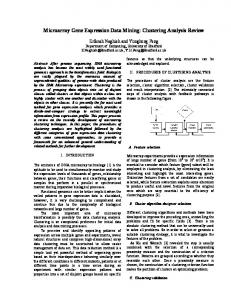
Given the two sets of row and column clusters, biclusters are assembled by considering all possible couples of row-columns clusters in such lists and by selecting only the couples of clusters that can mutually generate each other. More in details, consider a specific couple bij =< ri , cj >, we consider bij as a valid bicluster if and only if the clusters obtained by clustering the sub-matrix A[ri , :] along the columns contains cj and vice versa. Here, A[ri , :] represents the sub-matrix of the input data obtained by considering only the subset of rows contained in the cluster ri and all the columns. This condition effectively avoids that couples of clusters that do not form a biclusters in the input matrix are assembled together. To further clarify this point, Figure 1 reports an example of a couple of clusters that do form a bicluster in the input data. Specifically Figure 1(a) shows the input data and the row and column clusters that we want to test. Let’s consider the column submatrix (Figure 1(b)), clustering along the rows we obtain three clusters that include the input row cluster. The same happens when we consider the row submatrix of Figure 1(c), hence we can conclude that the input cluster couple does form a bicluster of the input data, as Figure 1(d) shows. On the other hand, Figure 2 reports an example of a couple that does not form a bicluster. Here, we consider the same input data matrix as before but a different cluster couple as Figure 2(a) shows. Running the test for this couple we can see that by considering the row submatrix we do obtain the input column cluster (2(b)). However, when we consider the column submatrix we can not find the input row cluster (2(c)). Therefore this cluster couple would not pass our test and in fact this is not a bicluster of the input data as Figure 2(d) shows.

(a)

(c)

(b)

(d)

Fig. 1. Couple of clusters that form a bicluster: (a) Input data and the couple of clusters to test. (b) Submatrix considering the column cluster. (c) Submatrix considering the row cluster. (d) Bicluster formed by the couple of clusters.

20

A. Farinelli, M. Denitto, and M. Bicego

(a)

(c)

(b)

(d)

Fig. 2. Couple of clusters that do not form a bicluster: (a) Input data and the couple of clusters to test. (b) Submatrix considering the row cluster. (c) Submatrix considering the column cluster. (d) Submatrix formed of row and columns clusters, which is not a bicluster of the input data.

Having described our approach the next session will report and discuss results obtained in the empirical evaluation of our method.

4

Experimental Evaluation

The methodology proposed in this paper has been tested in a synthetic benchmark ([22]), which includes synthetic expression matrices, perturbed with different schemes1 . In this setting, biclusters represent transcription modules; these modules are defined by (i) a set G of genes regulated by a set of common transcription factors, and (ii) a set C of conditions in which these transcription factors are active. In the original paper two scenarios are considered, one with non overlapping biclusters and one with overlapping biclusters. Here we consider only non overlapped biclusters, since the CTWC scheme does not permit to extract overlapped biclusters. In the experiments, 10 non-overlapping transcription modules, each extending over 10 genes and 5 conditions, emerge. Each gene is regulated by exactly one transcription factor and in each condition only one transcription factor is active. The corresponding datasets contain 10 implanted biclusters and have been used to study the effects of noise on the performance of the biclustering methods. The accuracy of the biclustering has been assessed with the so-called Gene Match Score [22], which reflects the similarity of the biclusters obtained by an 1

All datasets may be downloaded from: www.tik.ee.ethz.ch/sop/bimax

Biclustering of Expression Microarray Data Using Affinity Propagation

21

algorithm and the original known biclustering (it varies between 0 and 1, the higher the better the accuracy), for all details on the datasets and the evaluation protocol please refer to [22]. Even if our proposed approach is also able to extract biclusters with an average expression value close to zero, in this setting we remove such groups, in order to adapt our results to the synthetic evaluation of [22]. The proposed approach has been tested using as similairty the negative Euclidean distance and the Pearson coefficient, the latter being a very common choice in the microarray analysis scenario. Results were qualitatively and quantitatively really similar, thus here we report only those with the negative Euclidean distance. As for the stability threshold, after a preliminary evaluation we have found that a 50% value represents a good compromise between quality of clusters and level of details. Concerning the affinity propagation clustering algorithm, it is well known that setting the preferences may be crucial in order to obtain a proper clusterization [10]. Even if some sophisticated solutions have been proposed ( e.g. [26]) the most widely used approach is to set all the preferences as the median value of the similarity matrix [10]. Here we slightly enlarge the scope of this rule, by also setting as preferences the median +/- the Median Absolute Deviation (MAD) (which represents a robust estimator of the standard deviation [13]), defined, for a given population {xi } with median med, as M AD = mediani {|xi − med|}

(3)

The results are reported in Fig. 3, for the different initialization of the preference values. Following [22], we report both bicluster relevance (i.e., to what extent the generated biclusters represent true biclusters), and module recovery (i.e., how well true biclusters are recovered). Reported results support two main conclusions: i) the method performs extremely well on this dataset, with a worst case performance that still provides 91% accuracy. By comparing these results with those published in [22,2], we can

Recovery

Relevance

1

0.98

0.98

0.96

0.96

GMS

GSM

1

0.94

0.94

0.92

0.92

Median

Median

Median + MAD

Median + MAD

Median − MAD

Median − MAD 0.9

5

10

15 noise level

(a)

20

25

0.9

5

10

15 Noise Level

20

25

(b)

Fig. 3. Results on the synthetic dataset: (a) bicluster relevance, (b) module recovery

22

A. Farinelli, M. Denitto, and M. Bicego

observe that our approach is very competitive with respect to the state of the art. ii) while in principle the initialization of preference values does make a difference in the AP method, the approach is not very sensitive to this parameter, reaching very good performances for preference values within the tested range (especially in the first four conditions). Moreover, it is worth noticing that the different performance of the three preference settings confirm the intuition that higher preference values lead to more clusters in AP. In fact, the reason why the median − M AD has worst average performance, in terms of recovery, is due to the fact that AP forms less clusters thus failing to detect some of the biclusters that are present in the data set when the level of noise increases. On the other hand, by setting higher preferences AP finds more clusters thus resulting in a GMS that is more robust to the increasing noise level while maintaining a very good level of relevance. As a further analysis, we tried to understand which kind of errors are produced by the approach. In particular, in Fig. 4 we reported the biclusters extracted

Fig. 4. Example of the result of the algorithm: the original expression matrix is shown in the top left corner, in the remaining boxes the obtained biclusters are displayed

Biclustering of Expression Microarray Data Using Affinity Propagation

23

by the proposed approach in one of the run of the algorithm, within the last condition. It is clear that almost all the biclusters have been obtained, there is just one which has been divided in two. Therefore, the elements are correctly grouped together (the algorithm does not group together expressions which are not supposed to be together), but oversegmentation occurs. This issue may be possibly faced by selecting the preferences in the AP clustering module in a more careful way.

5

Conclusions and Future Works

In this paper we propose a method to use Affinity Propagation [10] (a recently proposed, promising clustering techniques), to perform biclustering of expression microarray data. Our method builds on the CTWC biclustering scheme [11] and extends it in two main directions: i) we propose a stability criterion, inspired from the bootstrap method, which is suited for AP, and more general that the one used in the original version of CTWC. ii) we propose a method to automatically assemble couples of stable clusters into biclusters. We empirically evaluated our approach in a synthetic benchmark [22], and results show that our method is very competitive with respect to state of the art. Future work in this area includes two main research directions: i) testing the approach on real biological data sets to assess the practical significance of the approach, ii) investigate extensions of the approach to deal with overlapping biclusters.

References 1. Bay, A., Granitto, P.: Clustering gene expression data with a penalized graph-based metric. BMC Bioinformatics 12 (2011) 2. Bicego, M., Lovato, P., Ferrarini, A., Delledonne, M.: Biclustering of expression microarray data with topic models. In: Proceedings of the International Conference on Pattern Recognition, pp. 2728–2731 (2010) 3. Bicego, M., Lovato, P., Oliboni, B., Perina, A.: Expression microarray classification using topic models. In: ACM Symposium on Applied Computing (Bioinformatics and Computational Biology track) (2010) 4. Bishop, C.: Pattern Recognition and Machine Learning. Springer, Heidelberg (2006) 5. Blei, D., Ng, A., Jordan, M.: Latent Dirichlet allocation. Journal of Machine Learning Research 3, 993–1022 (2003) 6. Br¨ andle, N., Bischof, H., Lapp, H.: Robust DNA microarray image analysis. Machine Vision and Applications 15, 11–28 (2003) 7. Chiu, T.Y., Hsu, T.C., Wang, J.S.: Ap-based consensus clustering for gene expression time series. In: Proc. Int. Conf. on Pattern Recognition, pp. 2512–2515 (2010) 8. de Souto, M., Costa, I., de Araujo, D., Ludermir, T., Schliep, A.: Clustering cancer gene expression data: A comparative study. BMC Bioinformatics 9 (2008)

24

A. Farinelli, M. Denitto, and M. Bicego

9. Felsenstein, J.: Confidence limits on phylogenies: an approach using the bootstrap. Evolution 39, 783–791 (1985) 10. Frey, B., Dueck, D.: Clustering by passing messages between data points. Science 315, 972–976 (2007) 11. Getz, G., Levine, E., Domany, E.: Coupled two-way clustering analysis of gene microarray data. Proc. Natl. Acad. Sci. USA 97(22), 12079–12084 (2000) 12. Givoni, I., Frey, B.: A binary variable model for affinity propagation. Neural Computation 21(6), 1589–1600 (2009) 13. Hampel, F., Rousseeuw, P., Ronchetti, E., Stahel, W.: Robust Statistics: the Approach Based on Influence Functions. John Wiley & Sons (1986) 14. Hofmann, T.: Unsupervised learning by probabilistic latent semantic analysis. Machine Learning 42(1-2), 177–196 (2001) 15. Jain, A., Dubes, R.: Algorithms for clustering data. Prentice-Hall (1988) 16. Kiddle, S., Windram, O., McHattie, S., Mead, A., Beynon, J., Buchanan-Wollaston, V., Denby, K., Mukherjee, S.: Temporal clustering by affinity propagation reveals transcriptional modules in arabidopsis thaliana. Bioinformatics 26(3), 355–362 (2010) 17. Kschischang, F., Frey, B., Loeliger, H.A.: Factor graphs and the sum-product algorithm. IEEE Transactions on Information Theory 47(2), 498–519 (2001) 18. Lee, J.W., Lee, J.B., Park, M., Song, S.: An extensive comparison of recent classification tools applied to microarray data. Computational Statistics & Data Analysis 48(4), 869–885 (2005) 19. Leone, M., Weigt, S., Weigt, M.: Clustering by soft-constraint affinity propagation: applications to gene-expression data. Bioinformatics 23(20), 2708–2715 (2007) 20. Madeira, S., Oliveira, A.: Biclustering algorithms for biological data analysis: a survey. IEEE Trans. on Computational Biology and Bioinformatics 1, 24–44 (2004) 21. Perina, A., Lovato, P., Murino, V., Bicego, M.: Biologically-aware Latent Dirichlet Allocation (BaLDA) for the Classification of Expression Microarray. In: Dijkstra, T.M.H., Tsivtsivadze, E., Marchiori, E., Heskes, T. (eds.) PRIB 2010. LNCS, vol. 6282, pp. 230–241. Springer, Heidelberg (2010) 22. Prelic, A., Bleuler, S., Zimmermann, P., Wille, A., Buhlmann, P., Gruissem, W., Hennig, L., Thiele, L., Zitzler, E.: A systematic comparison and evaluation of biclustering methods for gene expression data. Bioinformatics 22(9), 1122–1129 (2006) 23. Rogers, S., Girolami, M., Campbell, C., Breitling, R.: The latent process decomposition of cdna microarray data sets. IEEE/ACM Transactions on Computational Biology and Bioinformatics 2(2), 143–156 (2005) 24. Statnikov, A., Aliferis, C., Tsamardinos, I., Hardin, D., Levy, S.: A comprehensive evaluation of multicategory classification methods for microarray gene expression cancer diagnosis. Bioinformatics 21(5), 631–643 (2005) 25. Valafar, F.: Pattern recognition techniques in microarray data analysis: A survey. Annals of the New York Academy of Sciences 980, 41–64 (2002) 26. Zhang, X., Wu, F., Zhuang, Y.: Clustering by evidence accumulation on affinity propagation. In: Proc. Int. Conf. on Pattern Recognition, pp. 1–4 (2008)