Biclustering of Expression Data Using Simulated Annealing∗ Kenneth Bryan, P´adraig Cunningham, Nadia Bolshakova Trinity College Dublin, College Green, Dublin 2, Ireland
[email protected]
Abstract In a gene expression data matrix a bicluster is a grouping of a subset of genes and a subset of conditions which show correlating levels of expression activity. The difficulty of finding significant biclusters in gene expression data grows exponentially with the size of the dataset and heuristic approaches such as Cheng and Church’s greedy node deletion algorithm are required. It is to be expected that stochastic search techniques such as Genetic Algorithms or Simulated Annealing might produce better solutions than greedy search. In this paper we show that a Simulated Annealing approach is well suited to this problem and we present a comparative evaluation of Simulated Annealing and node deletion on a variety of datasets. We show that Simulated Annealing discovers more significant biclusters in many cases.
1. Introduction In recent years the advent of DNA microarray technologies has revolutionised the study of gene expression. It is now possible to monitor the expression of thousands of genes in parallel over many experimental conditions (e.g. different patients, tissue types and growth environments), all within a single experiment (see Lander [13]). The results from these experiments are usually presented in the form of a data matrix in which rows represent genes and columns represent conditions. Each entry in the matrix is a measure of the expression level of a particular gene under a specific condition. Thorough analysis of these datasets aids in the annotation of genes of unknown function and the discovery of functional relationships between genes. This ultimately contributes to the elucidation of biological systems at a molecular level [3]. However mining this valuable information from such large volumes of data presents a far from trivial task. One of the main methods used thus far has been cluster analysis [8], [20], [7]. In this approach genes which show similar expression activity over the set of conditions are grouped together into clusters under the premise that these genes may be functionally related. Conditions too may be clustered enabling disease types such as cancers to be defined in terms of their unique expression profiles [17]. Gene expression datasets are continually growing in size as more experiments are carried out and as experimental capacity improves. With increasing size it becomes less likely that objects (genes) will retain similarity across all attributes (conditions) making clustering problematic. Furthermore it is not uncommon for the expression of genes to be highly similar under one set of conditions and yet independent under another set [2]. Clustering genes over a subset of conditions would be more beneficial in such cases. This approach has been termed biclustering and was first introduced to gene expression ∗
This research was sponsored by Science Foundation Ireland under grant number SFI-02/IN1/I111
1
analysis by Cheng and Church [6]. Since then the concept has been adopted in several studies in this field [14],[19],[12]. Cheng and Church identified the problem of finding significant biclusters as being NP-Hard and employed a greedy node deletion algorithm in their search. The review of biclustering algorithms for biological data analysis presented by Madeira and Oliveira [15] also identifies greedy search algorithms as a promising approach. Greedy search algorithms start with an initial solution and find a locally optimal solution by successive transformations that improve some fitness function. Simulated Annealing (SA) [11] improves on greedy search due to its potential to escape local minima (see section 3). In this paper we present a biclustering technique based on SA that improves on results produced by Cheng and Church’s node deletion algorithm (see section 2). We perform this evaluation on three datasets derived from human and yeast expression studies and show that our SA based solution finds more significant biclusters in each dataset (see section 5). The measure of significance we use is the mean squared residue function proposed by Cheng and Church. This is followed by a biological evaluation of the biclusters discovered by SA.
2. Biclustering Cheng and Church proposed the mean squared residue function to score sub-matrices and find biclusters within a gene expression matrix. This scoring of sub-matrices is based upon the concept of the residue score. In the sub-matrix IJ, the residue of an entry, aij , is defined to be: R(aij ) = aij − aIj − aiJ + aIJ
(1)
where aiJ is the mean of the ith row , aIj is the mean of the jth column and aIJ mean of the whole sub-matrix. This is a measure of how well the entry fits into that sub-matrix. The overall mean squared residue for the sub-matrix is given by: H(I, J) =
X 1 R(aij )2 |I||J| i∈I,j∈J
(2)
This is a measure of how well the rows and columns fit together or how well correlated the submatrix is. A well correlated sub-matrix, one with a low mean squared residue is referred to as a bicluster of that parent matrix. A perfectly correlated bicluster would have a score of zero. For a more detailed discussion on the mean squared residue scoring function see [6]. In the context of gene expression a bicluster of genes and conditions may represent an in vivo orchestration of expression to suit a common functional activity. Thus biclustering gene expression data may aid in the discovery and elucidation of such biological functional modules. It is important for these models to be as complete as possible and therefore the goal should be to find maximally sized biclusters. Cheng and Church proposed a greedy node deletion algorithm to find the maximally sized biclusters of a pre-defined low mean squared residue score (δ-biclusters). The algorithm works in a top-down manner beginning with the whole dataset and then proceeds to delete the rows or columns which most improve the mean squared residue score of the matrix. The first phase of the Church and Cheng algorithm is a multiple node deletion phase included for speed in which several row/columns are deleted simultaneously. However there is a possibility that multiple node deletion will overrun the δ threshold and affect accuracy so the single node deletion phase is only implemented in this study. Upon reaching the δ threshold a node addition phase is then carried out to add rows/columns which may have been missed. Inversely correlated rows, which may represent negatively regulated genes, are also added at this stage. A subsequent study [22] noted that as with other greedy searches there is a possibility that the system may become trapped at a locally good solution or local minimum so the global maximum or maximal δ-bicluster or is unlikely to be found.
3. Simulated Annealing Stochastic techniques which allow acceptance of reversals in fitness have been shown to improve on greedy approaches by performing more in-depth searches of feature space. Recently evolutionary optimization schemes have been employed with the mean squared residue function in the bicluster search problem [5], [1]. These attempts failed to find better solutions than the Church and Cheng technique in terms of bicluster size and instead focused on returning smaller sets of biclusters with high row variability. Simulated Annealing is a well established stochastic technique which was originally developed to model the natural process of crystallisation [16] and later adopted to solve optimisation problems[11]. Like a greedy search it accepts changes which lead to improvements in the fitness of a solution but also allows the probabilistic acceptance reversals in fitness. This probability is inversely proportional to the size of the reversal and also decreases as the search continues allowing eventual convergence on a solution. The probability of accepting a reversal is defined by Boltzman’s equation: ∆E P (∆E) ∝ e− T (3) Where ∆E is the difference in energy (fitness) between the old and new states and T is the temperature of the system. In the natural process the system cools logarithmically. However this is so time consuming that many simplified cooling schedules have been introduced for practical problem solving; the following linear cooling model is popular: T (k) =
T (k − 1) 1+σ
(4)
Where T (k) is the current temperature, T (k − 1) is the previous temperature and σ dictates the cooling rate. Simulated Annealing has been applied to such problems as the well known travelling salesman problem [4] and optimisation of wiring on computer chips [11]. Its application to biclustering gene expression data is a logical step given the drawbacks of current approaches.
4. Experimental Methods Our Simulated Annealing Biclustering (SAB) algorithm begins the search in a top-down manner with an initial solution comprising all rows and columns. Rows/columns are then added or deleted and the mean squared residue (see equation 2) is used as the fitness function to score these submatrices. The initial temperature of the system, T 0 , was chosen so as to initially allow 80 percent of reversals to be accepted as recommended in [18]. The annealing schedule used is of the type in equation 4 with σ = 0.1. This means that each subsequent temperature is approximately 0.9 times that of the previous temperature. The temperature is lowered after 10xN successful transformations or 100xN attempted transformations, where N is equal to the number of genes in the dataset. Upon reaching a δ-bicluster the size of this bicluster is then increased while maintaining the δ-score. When no improvements are possible the bicluster solution is then returned. SAB then performs a node addition phase on each bicluster to add inversely correlated rows and to allow better comparison with Cheng and Church’s node deletion. To prevent biclusters from being rediscovered in subsequent searches their entries are replaced with random numbers this masking is fully described in [6]. Three datasets were used to compare the node deletion technique with that of SAB. The first was the yeast dataset of 2,884 genes and 17 conditions used by Church and Cheng (see: http://arep.med.harvard.edu/biclustering/yeast.matrix). A human scleroderma dataset of 2,774 genes and 27 conditions from [21] (see:http://genome-www.stanford.edu/scleroderma/data.shtml) and Lymphoma dataset of 3,051 genes and 38 conditions from [9] were also used in the evaluation.
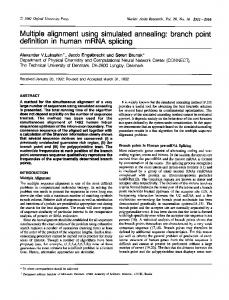
5. Evaluation of Biclustering Using Simulated Annealing There are two questions dealt with in the evaluation section. Firstly we investigate whether SAB can retrieve solutions closer to the global maximum than the Cheng and Church node deletion (CCND) approach i.e. larger δ-biclusters. The second question is whether biclusters discovered by SAB reflect in vivo functional modules. In this paper we use an annotated gene expression dataset to investigate whether SAB discovers such verifiable biclusters. 5.1. Comparative Evaluation with Node Deletion Cheng and Church carried out node deletion on the yeast dataset mentioned above and used a mean squared residue threshold (δ) of 300 (as determined by equation (2)). The SAB algorithm was applied to the same yeast dataset. In this study δ thresholds of 300, 200 and 100 were set and the size of the discovered biclusters compared in each case. SAB produces biclusters of at least 10 columns in width. To align the algorithms and ensure that the column size of the resultant biclusters does not bias the results an adjusted node deletion algorithm (CCND2) is also run in which the column size of resultant biclusters is set to 10. Figure 1(a) shows the size of the first bicluster found by CCND, CCND2 and SAB over the various δ thresholds for the yeast dataset. Figure 1(b) shows the second bicluster discovered when the first was masked with random numbers as described in [6]. SAB performed better than CCND and CCND2 for all delta scores locating larger δ-biclusters in all cases.
(a)
Comparison of Biclustering Algortihms (Yeast Data)
CCND2
Comparison 2nd Bicluster (Yeast Data)
CCND2
SAB
18000
9000
16000
8000
14000
7000
Bicluster Size
Bicluster Size
CCND
(b)
12000 10000 8000 6000
SAB
6000 5000 4000 3000
4000
2000
2000
1000 0
0
delta = 300
delta = 200
delta = 100
delta = 300
delta = 200
delta = 100
Figure 1. (a) Comparisons of Cheng and Church’s node deletion algorithm (CCND), our adjusted node deletion algorithm (CCND2) and Simulated Annealing Biclustering (SAB) using the yeast dataset over δ -scores of 300, 200 and 100. (b) The second biclusters found by CCND2 and SAB.
The results for all three data sets are shown in Table 1, numbers in bold mark the best biclusters. SAB performed better than CCND discovering larger δ-biclusters in all cases. The CCND2 algorithm performed better than the original CCND but even so SAB still performed better in most cases. In Table 1 it can be seen that SAB performs better than CCND2 discovering a larger first bicluster in 4/9 cases and draws in a further 3 cases. SAB performed best in discovering the second biclusters in 6/9 cases over the three datasets.
Yeast
Scleroderma
Lymphoma
δ-Score 300 200 100 300 200 100 300 200 100
CCND CCND2 SAB Bicluster 1 (Rows x Cols) 15165 15750 16460 8463 9540 10360 2520 2700 2940 13590 18260 18230 7296 12920 13210 2730 5170 5140 1344 3320 3220 1032 2510 2460 851 1780 1790
CCND 9012 4972 1260 4320 7876 1570 518 300 136
CCND2 Bicluster 2 3930 2630 830 6780 3290 830 1740 1370 1050
SAB 8320 3860 1390 6310 4030 850 1810 1200 810
Table 1. The first two biclusters discovered in each dataset for δ -score thresholds of 300, 200 and 100. The largest δ -biclusters are marked in bold (draws are marked when there is a very small size difference < 0.005 %). Italicised values for the second bicluster cannot be compared directly as they are taken from a significantly larger initial set.
Bicluster 1
No. of Genes 81
Bicluster 2
59
Dominant Functional Category Ribosomal Proteins(96) Glycolysis/Glucogenisis(26) Basal Transcription Factors(10) Nucleotide Metabolism(81)
Genes in Functional Category 61 5 6 16
Lift Value 4.31 5.7 5.51 1.84
Table 2. Known functional modules found by SAB in the annotated gene dataset. See text.
5.2. Biological Interpretation A more practical way to evaluate SAB is to use a fully annotated dataset. Of the 2884 genes in the yeast dataset 550 can be annotated from the online database called Kyoto Encyclopaedia of Genes and Genomes, KEGG (http://www.genome.jp/kegg/genes.html). Ideally the biclusters in such a dataset would then reflect in vivo groups of genes known to be functionally related. A δ-score of 100 was chosen as the mean squared residue threshold. In Table 5.2 it can be seen that the first bicluster discovered from this annotated dataset is rich in genes from the ribosomal functional category. The second bicluster contains transcription factors and genes involved nucleotide metabolism. These genes are the main regulators of protein production and gene expression in the cell. The statistical significance of discovering this grouping is given by the lift score (see [10]). This value measures whether a particular grouping is over-represented or not. A lift score above 1 for a particular group within a sample suggests that there is some positive bias in this group’s selection. Further biclusters contained correlating genes but no dominating known functional categories, so are not listed.
6. Conclusions & Future Work Using SAB we have shown that stochastic methods have the potential to give improved results for the bicluster search problem. We have shown that SAB performs better than the Cheng and Church’s original node deletion algorithm in that it discovers larger δ-biclusters. SAB also performs better when compared to our improved version of the node deletion algorithm. When applied to the annotated yeast dataset SAB discovers recognizable classes of genes. SAB works in top-down manner with the mean squared residue function promoting the deletion of rows/columns which do not fit in with the trends in the dataset. As a result biclusters may be biased towards core regulatory
genes which govern the general state of gene expression the cell. Outlying biclusters would tend to have their ill-fitting rows/columns deleted early on in the search. Evidence of this can be seen in the nature of the classes of genes in biclusters 1 and 2 from the annotated set. Perhaps this bias could be harnessed to discover regulatory genes within gene expression data. Although a bottom-up search approach using the mean squared residue as a fitness function would probably not find such large biclusters it would perhaps promote more variability in the classes of genes it discovers. A next step could be to use Simulated Annealing in a bottom-up search in a bid to discover smaller more natural biclusters which may better reflect the natural state or organisation in an organism.
References [1] J. S. Aguilar-Ruiz and F. Divina. Evolutionary computation for biclustering of gene expression. In Proc. ACM symposium on Applied computing, page to appear. ACM Press, 2005. [2] A. Ben-Dor, B. Chor, R. Karp, and Z. Yakini. Discovering local structure in gene expression data: the orderpreserving submatrix problem. Journal of Computational. Biology, 10(3-4):373–84, 2003. [3] D. Berrer, W. Dubitzky, and S. Draghici. A Practical Approach to Microarray Data Analysis, chapter 1, pages 15–19. Kluwer Academic Publishers, 2003. [4] K. Binder and D. Stauffer. A simple introduction to Monte Carlo simulations and some specialized topics, chapter Applications of the Monte Carlo Method in Statistical Physics, pages 1–36. Spring-Verlag, Berlin, 1985. [5] S. Bleuler, A. Preli´c, and E. Zitzler. An EA framework for biclustering of gene expression data. In CEC, pages 166–173, Piscataway, NJ, 2004. IEEE. [6] Y. Cheng and G. M. Church. Biclustering of expression data. In Proc.ISMB, pages 93–103, 2000. [7] I. S. Dhillon, S. Mallela, and D. S. Modha. Information theoretic co-clustering. In Proc. ACM SIGKDD International Conference on Knowledge Discovery and Data Mining, 2003. [8] M. B. Eisen, P. T. Spellman, P. O. Brown, and D. Botstein. Cluster analysis and display of genome-wide expression patterns. Proc. of the National Academy of Sciences, USA, 8(95):14863–8, 1998. [9] T. Golub, D. Slonim, P. Tamayo, C. Huard, M. Gaasenbeek, J. Mesirov, H. Coller, M. Loh, J. Downing, M. Caligiuri, C. Bloomfield, and E. Lander. Molecular classification of cancer: class discovery and class prediction by gene expression monitoring. Science, 286(5439):531–537, 1999. [10] J. Han and M. Kamber. Data Mining: Concepts and Techniques, chapter 6. Morgan Kaufmann Publishers, 2000. [11] S. Kirkpatrick, C. D. Gelatt, and M. P. Vecchi. Optimization by simulated annealing. Science, 220(4598):671–680, 1983. [12] Y. Kluger, R. Basri, J. T. Chang, and M. Gerstein. Spectral biclustering of microarraydata: Coclustering genes and conditions. Genome Research, 13:703–716, 2003. [13] E. S. Lander. Array of hope. Nature Genetics., 21:3–4, 1999. [14] L. Lazzeroni and A. Owen. Plaid models for gene expression data. Statistica Sinica, 12:61–86, 2002. [15] S. C. Madeira and A. L. Oliveira. Biclustering algorithms for biological data analysis: A survey. IEEE/ACM Transactions on Computational Biology and Bioinformatics, 1(1):24–45, 2004. [16] N. Metropolis, A. W. Rosenbluth, M. N. Rosenbluth, A. H. Teller, and E. Teller. Equations of state calculations by fast computing machines. Journal of Chemical Physics, 21:1087–1092, 1958. [17] S. L. Pomeroy, P. Tamayo, M. Gaasenbeek, L. M. Sturla, M. Angelo, M. E. McLaughlin, J. Y. Kim, L. C. Goumnerova, P. Black, C. Lau, J. C. Allen, D. Zagzag, J. M. O. andT Curran, C. Wetmore, J. A. Biegel, T. Poggio, S. Mukherjee, R. Rifkin, A. Califano, D. Stolovitzky, D. Louis, J. Mesirov, E. Lander, and T. Golub. Prediction of central nervous system embryonal tumour outcome based on gene expression. Nature, 24(415):436–42, 2002. [18] B. Preiss. Data Structures and Algorithms with Object-Oriented Design Patterns in Java. John wiley and Sons, 1999. [19] A. Tanay, R. Sharan, and R. Shamir. Discovering statistically significant biclusters in gene expression data. Bioinformatics., 18:36–44, 2002. [20] S. Tavazoie, J. D. Hughes, M. Campbell, R. J. Cho, and G. M. Church. Systematic determination of genetic network architecture. Proceedings of the National Academy of Sciences, USA., 22(3):281–5, 1999. [21] M. L. Whitfield, D. R. . Finlay, J. I. Murray, O. Troyanskaya, J.-T. Chi, A. Pergamenschikov, T. McCalmont, P. O. Brown, D. Botstein, and M. K. Connolly. Systemic and cell type-specific gene expression patterns in scleroderma. Proc. of the National Acadaemy of Sciences, 100(21):12319–12324, 2003. [22] J. Yang, H. Wang, W. Wang, and P. Yu. Enhanced biclustering on expression. In IEEE Third Symposium on Bioinformatics and Bioengineering. 2003.