Bidirectional Mining of Non-Redundant Recurrent Rules from a Sequence Database David Lo1 , Bolin Ding2 , Lucia1 , Jiawei Han2 1
School of Information Systems, Singapore Management University Department of Computer Science, University of Illinois at Urbana-Champaign Emails:
[email protected],
[email protected],
[email protected],
[email protected] 2
Abstract—We are interested in scalable mining of a nonredundant set of significant recurrent rules from a sequence database. Recurrent rules have the form “whenever a series of precedent events occurs, eventually a series of consequent events occurs”. They are intuitive and characterize behaviors in many domains. An example is the domain of software specification, in which the rules capture a family of properties beneficial to program verification and bug detection. We enhance a past work on mining recurrent rules by Lo, Khoo, and Liu to perform mining more scalably. We propose a new set of pruning properties embedded in a new mining algorithm. Performance and case studies on benchmark synthetic and real datasets show that our approach is much more efficient and outperforms the state-ofthe-art approach in mining recurrent rules by up to two orders of magnitude.
I. I NTRODUCTION Data mining has been shown useful in various domains including finance, marketing, bioinformatics and recently software engineering, e.g., [11], [17]. Many valuable data sources are in sequential formats ranging from logs, transaction histories, medical histories, program traces, and many more. To analyze sequential data, Lo et al. propose recurrent rules stating: “Whenever a series of events occurs, eventually another series of events occurs”. Recurrent rules capture temporal constraints that repeat a substantial number of times both within a sequence and across multiple sequences [18]. The rule format is general and is not limited by look-ahead limit or window-width constraint. This enables the rule to capture significant candidates for not only temporal shortdistance but also long-distance cause-and-effect relationships in a dataset. There are many instance of recurrent rules in day-to-day settings: 1. Resource Locking Protocol: Whenever a lock is acquired, eventually it is released. 2. Internet Banking: Whenever a connection is made and an authentication is completed and fund transfer command is issued, eventually the fund is transferred. 3. Network Protocol: Whenever an HDLC connection is made and an acknowledgement is received, eventually a disconnection message is sent and an acknowledgement is received. Zooming into the domain of software specification and verification, recurrent rules correspond to a family of program properties useful for program verification (c.f., [9]). The first example given above is a program property. Research
in software verification addresses approaches to check the correctness of a software with respect to a formal specification which often corresponds to a set of properties (c.f., [6]). However, documented specifications might often be outdated or missing due to software evolution, reluctance in writing formal specifications and short-time-to-market cycle of software development (c.f., [7], [5]). There are past studies on mining association rules from sets of items [2]. These studies are later extended to mine for sequential patterns and episodes that consider ordering among events in sequences [3], [20]. Rules can be formed from both sequential patterns and episodes [24], [20]. Different from a pattern, a rule expresses a constraint involving its premise (i.e., pre-condition) and consequent (i.e., post-condition). These constraints are needed for their potential usages in filtering erroneous sequences, detecting outliers, etc. However, rules generated from sequential patterns and episodes have different semantics from recurrent rules. A sequential rule pre → post states: “Whenever a sequence is a super-sequence of pre it will also be a super-sequence of pre concatenated with post”. An episode rule pre → post states: “Whenever a window is a super-sequence of pre it will also be a super-sequence of pre concatenated with post”. To illustrate the differences, consider the following sequences: Seq ID. S1 S2
Sequence ⟨lock, use, use, use, use, unlock⟩ ⟨lock, use, use, use, use, unlock, lock, lock, exit⟩
From sequence S1, episode rule mining with a window size of two is not able to mine the rule: “lock must be followed by unlock” as the two events are separated by more than two events. From sequences S1 and S2, sequential rule mining would report “lock must be followed by unlock with a perfect confidence or likelihood (2 out of 2 cases)” despite the last two lock operations in S2 are not paired with any subsequent unlock operations. Considering both S1 and S2, recurrent rule mining would report “lock is followed by unlock in 2 out of 4 cases”. Recurrent rules generalize sequential rules where for each rule, multiple occurrences of the rule’s premise and consequent both within a sequence and across multiple sequences are considered. Recurrent rules generalize episode rules by allowing precedent and consequent events to be separated by
an arbitrary number of events in a sequence database. Also, a set of sequences rather than a single sequence is considered during mining. Furthermore, rather than mining all rules we mine a non-redundant set of rules. Recurrent rules could be formalized in Linear Temporal Logic (LTL) [14]. LTL has been widely studied and many tools have been built on top of it, e.g., [6], [16]. Model checker is one of them [6]. It allows verifying correctness of safety critical systems based on the satisfaction of rules and properties formalized in LTL. The new semantics of recurrent rules, as compared to association, sequential and episode rules, necessitates new pruning strategies and algorithms that utilize these strategies to efficiently mine for recurrent rules. The pioneer work on recurrent rules is a past study by Lo, Khoo and Liu in [18]. However, with the growth in the size of data currently available, there is a need for a more scalable algorithm. On larger datasets or lower support thresholds, we find that there is a need to enhance the scalability of the algorithm in [18]. This work fills this gap by proposing a more scalable algorithm that embeds new pruning properties to mine recurrent rules more efficiently. Our approach works in several steps: 1. Mining pruned pre-conditions, 2. Mining pruned post-conditions, 3. Rule formation, and 4. Redundant rules removal. A number of new pruning strategies and a new data structure are employed for efficient mining of a non-redundant set of recurrent rules. Under a condition which holds in many cases, the complexity of the proposed algorithm is smaller by an exponential factor than the complexity of the one proposed in [18] (see Section VI-D). Performance study conducted on benchmark datasets, both synthetic and real, shows that runtime is improved by up to 134 times. We also conducted a case study on a dataset of real software traces extracted from multiple user interactions with an instant messaging application. The outline of this paper is as follows. In Section II, we discuss related work. Section III presents recurrent rule semantics in Linear Temporal Logic (LTL). Section IV describes some notations and definitions used in subsequent sections. Section V presents various theorems and properties used to prune search spaces. Section VI presents our algorithm and compares it with [18]. Section VII describes our performance study and case study. Finally, we conclude and describe future work in Section VIII. II. R ELATED W ORK In this section, we discuss closely related past studies and compare them with our approach. Past Studies on Temporal Logics. In this work we mine recurrent rules, which is under the family of Linear Temporal Logic properties [14]. Temporal logics itself has been widely used for various purposes ranging from specifying communication protocols among agents or models of agents’ behaviors [15], modeling bio-molecular interactions [21], querying XML documents [4], supporting historical databases [28], verifying correctness of systems [6], etc. Many studies described
above use temporal logics to accomplish a particular task. Different from these past studies, our goal is to mine temporal logic expressions automatically from datasets. Mining Frequent Itemsets & Association Rules. Association rule mining is first proposed by Agrawal and Srikant in [2]. Association rule captures a relationship among items in a set, where the ordering of items is irrelevant. Association rules are generated by post-processing frequent itemsets. Notions of support and confidence are used as measures to distinguish significant rules. There are many work extending association rule mining, of special interest are work on closed frequent itemsets (e.g., [22]) and non-redundant association rules (e.g., [27]). Different from association rules, recurrent rules express ordering constraints among events in a sequence database. Due to this difference, pruning properties, suitable mining algorithms and the notion of rule redundancy are different. Mining Patterns & Rules from Sequences. Sequential pattern mining [3], [23] discovers patterns that are supported by a significant number of sequences. A pattern is supported by a sequence if it is a sub-sequence of it. To remove redundant patterns, closed sequential pattern mining was proposed by Yan et al. [26] and improved by Wang and Han [25]. Spiliopoulou proposed the generation of sequential rules from sequential patterns [24]. Recurrent rules generalize sequential rules by considering multiple occurrences of the premise and consequent events within a sequence and across multiple sequences in the database. This generalization is significant since the precedent and consequent events of a rule can potentially appear repeatedly in a sequence. Considering program execution traces, due to loops and recursion, it is common to see program properties observed repeatedly in a trace. Mannila et al. performed episode mining to discover frequent episodes within a sequence of events [20]. An episode is defined as a series of events occurring relatively close to one another (i.e. they occur at the same window). An episode is supported by a window if it is a sub-sequence of the series of events appearing in the window. There are many extensions of the work. Harms et al. mine for constrained episode rules where the distance between the precedent and consequent of a rule is further limited by a value smaller than the overall window size [12]. Garriga extends Mannila et al.’s work to replace a fixed-window size with a gap constraint between one event to the next in an episode [10]. Recurrent rules generalize rules formed from episodes by allowing precedent and consequent events to be separated by an arbitrary number of events. This generalization is significant since precedent and consequent events might possibly be separated by an arbitrary number of events in sequences. For example, useful program properties, such as: ‘acquiring of a lock (lock) is eventually followed by its release (unlock)’, or ‘an opened file (open) is eventually closed (closed)’ (c.f [17], [18]), often have their associated events occur at some arbitrary distance away from one another in an execution trace. Also, we analyze a sequence database and mine non-redundant rules. In [17], Lo et al. proposed iterative patterns to discover
TABLE I LTL E XPRESSIONS AND THEIR M EANINGS F (unlock) Meaning: Eventually unlock is called XF (unlock) Meaning: From the next event onwards, eventually unlock is called G(lock → XF (unlock)) Meaning: Globally whenever lock is called, then from the next event onwards, eventually unlock is called G(main → XG(lock → (→ XF (unlock → XF (end))))) Meaning: Globally whenever main followed by lock are called, then from the next event onwards, eventually unlock followed by end are called TABLE II RULES AND THEIR LTL E QUIVALENCES Notation a→b ⟨a, b⟩ → c a → ⟨b, c⟩ ⟨a, b⟩ → ⟨c, d⟩
LTL Notation G(a → XF b) G(a → XG(b → XF c)) G(a → XF (b ∧ XF c)) G(a → XG(b → XF (c ∧ XF d)))
software specifications, which are defined based on the semantics of Message Sequence Charts (MSC). In [8], Ding et al. proposed an approach to mine for repetitive sub-sequences. Our work could be viewed as an extension of their approaches to mine for repetitive rules following the semantics of Linear Temporal Logics. In the software domain, LTL (but not MSC) is one of the most widely-used formalism for program verification (i.e., ensuring correctness of a software system) [6]. Since the underlying target formalisms and semantics are different, both the search space pruning strategies and the mining algorithm needed to efficiently mine recurrent rules are very different from those used in the past studies in [17] and [8]. Mining recurrent rules is first proposed in [18]. In this work, we speed up the mining process further. We propose new pruning strategies and a new algorithm that embed the strategies into an effective approach to prune search space. Under a condition which holds in many cases, the complexity of our approach is exponentially better than the complexity of the approach in [18] (see Section VI-D). Furthermore, our empirical evaluation shows that our approach is able to outperform [18] by up to 2 orders of magnitude. III. RULE S EMANTICS IN LTL Our mined rules can be expressed in Linear Temporal Logic (LTL) [14]. LTL is a logic that specifies properties of a sequence (i.e., a series of events). There are a number of LTL operators, among which we are only interested in the operators: ‘G’,‘F’, and ‘X’. The operator ‘G’ specifies that globally for every event in a sequence a certain property holds. The operator ‘F’ specifies that a property holds either at the current event or finally (or eventually) in one of the subsequent events in a sequence. The operator ‘X’ specifies that a property holds at the next event. Some examples are listed in Table I. Our mined rules state whenever a series of precedent events occurs eventually another series of consequent events also occurs. A mined rule denoted as pre → post, can be mapped to its corresponding LTL expression. Examples of such correspondences are shown in Table II. Note that although the operator ‘X’ might seem redundant, it is needed
to specify rules such as ⟨a⟩→⟨b, b⟩ where the ‘b’s refer to different occurrences of ‘b’. The set of LTL expressions corresponding to the set of recurrent rules and are minable by our mining framework is shown in Backus-Naur Form (BNF) as follows: rules := prepost := post :=
G(prepost) event → post|event → XG(prepost) XF (event)|XF (event ∧ XF (post))
Example 1: To illustrate the semantics of recurrent rules, consider a sequence: S = ⟨main, lock, use, unlock, lock, end⟩ The LTL property corresponding to the rule ⟨main, lock⟩ → ⟨unlock, end⟩ is the property G(main → XG(lock → XF (unlock ∧ XF (end)))). This property is violated by S as the second occurrence of lock is not eventually followed by unlock and end. Note however, the property corresponding to ⟨main, lock, use⟩ → ⟨unlock, end⟩, which is G(main → XG(lock → XG(use → XF (unlock ∧ XF (end))))) is satisfied. This is the case since the second occurrence of lock immediately before end in S is not followed by a use. IV. N OTATIONS & D EFINITIONS This section presents some preliminary notations and definitions pertinent to mining recurrent rules. Many of these are taken from [18]. A. Basic Notations Let I be a set of distinct events considered. The input to our mining problem is a sequence database denoted as SeqDB = {S1 , S2 , . . . , S|SeqDB| }. Each sequence is an ordered list of events, denoted as ⟨e1 , e2 , . . . , eend ⟩ where ei ∈ I. We define a pattern P to be a series of events. We use first(P ) and last(P ) to denote the first and last event of P respectively. A pattern P1 ++P2 denotes the concatenation of patterns P1 and P2 , also said to be the forward extension of P1 or backward extension of P2 . A pattern P1 = ⟨e1 , e2 , . . . , en ⟩ is a subsequence (sub-pattern) of another pattern P2 = ⟨e′1 , e′2 , . . . , e′m ⟩ (or, P2 is a super-pattern of P1 ) if there exists integers 1 ≤ i1 < i2 < . . . < in ≤ m such that e1 = e′i1 , e2 = e′i2 , · · · , en = e′in (denoted as P1 ⊑ P2 , or P1 < P2 if they are not equal). Each recurrent rule R has the form Rpre → Rpost , where Rpre and Rpost are two series of events (i.e., two patterns). Rpre is referred to as the premise or pre-condition of the rule, while Rpost is referred to as the consequent or post-condition of R. B. Concepts and Problem Statement In this subsection, we discuss various concepts and definitions and define our problem statement. We use the database in Table III as our running example throughout this paper. Each recurrent rule we mine expresses:
TABLE III E XAMPLE S EQUENCE DATABASE – SeqDB Seq ID. S1 S2
Sequence ⟨a, b, e, c, b, d, c, d⟩ ⟨a, c, b, e, a, e, d, c, b, d⟩
“Whenever a series of events has just occurred at a point in time (i.e. a temporal point), eventually another series of events occurs” From the above semantics, to generate recurrent rules, we need to “peek” at interesting temporal points and “see” what series of events are likely to occur next. We will first formalize the notion of temporal points and occurrences. Definition 4.1 (Temporal Points & Prefixes & Suffixes): Consider a sequence S of the form ⟨a1 , a2 , . . . , an ⟩. All events in S are indexed by their positions in S, starting from 1 (e.g., S[2] = a2 ). These positions are called temporal points in S. For a temporal point j, the first j events ⟨a1 , . . . , aj ⟩ is the j-prefix of S; the last j events ⟨an−j+1 , . . . , an ⟩ is the j-suffix of S. Definition 4.2 (Occurrences & Instances): Given a pattern P and a sequence S, an occurrence of P in S is defined to be a temporal point j, such that the j-prefix of S is a supersequence of P and last(P )=S[j]. Each of such j-prefixes is said to be an instance of the pattern P in S, i.e., it is a super-sequence of P and last(P ) is indexed by j. An instance of P in S is minimum iff it is the shortest one, i.e., there is no k < j such that k-prefix of S is an instance of P . Example 2: Consider a pattern P ⟨a, b⟩ and the sequence S1 in the example database in Table III (i.e., ⟨a, b, e, c, b, d, c, d⟩). Temporal points {2, 5} are the occurrences of P in S1 , and the corresponding instances are ⟨a, b⟩ and ⟨a, b, e, c, b⟩, where the instance ⟨a, b⟩ is the minimum one. Definition 4.3 is a standard database projection (c.f. [26], [25]) capturing series of events occurring after the first temporal point. Definition 4.4 is a new type of projection capturing series of events occurring after each temporal point introduced in [18]. Definition 4.3 (Projection & Sequence Support): A database projected on a pattern P is defined as: SeqDB P = {(i, sx) | Si ∈ SeqDB , satisfying Si = px++sx, and px is the minimum instance of P in Si , i.e., px is the shortest prefix of Si containing P }. For a pattern P , we define the sequence support sup(P ,SeqDB ) to be the size of SeqDB P (or equivalently, the number of sequences in SeqDB containing P ). Reference to the database is omitted if it is clear from the context. Definition 4.4 (All-Projection & Instance Support): A database all-projected on a pattern P is defined as: SeqDB all P = {(i, sx) | Si ∈ SeqDB , satisfying Si = px++sx, and px is an instance of P in Si }. For a pattern P , we define the instance support sup all (P, SeqDB ) to be the size of SeqDB all P (or equivalently, the total number of instances of P in all sequences of SeqDB ).
Reference to the database is omitted if it is clear from the context. Example 3: To illustrate the above concepts, we list the projected and all-projected database SeqDB w.r.t. ⟨a, b⟩ in Table III. From the support notations, we have sup(⟨a, b⟩, SeqDB ) = |SeqDB ⟨a,b⟩ | = 2, sup all (⟨a, b⟩, SeqDB ) = |SeqDB all ⟨a,b⟩ | = 4. TABLE IV P ROJECTION AND A LL -P ROJECTION Projection SeqDB ⟨a,b⟩ (1, ⟨e, c, b, d, c, d⟩) (2, ⟨e, a, e, d, c, b, d⟩)
All-Projection SeqDB all ⟨a,b⟩ (1, ⟨e, c, b, d, c, d⟩) (1, ⟨d, c, d⟩) (2, ⟨e, a, e, d, c, b, d⟩) (2, ⟨d⟩)
The two projection methods associated notions of sup and sup all are different. Specifically, sup all reflects the number of occurrences of P in SeqDB rather than the number of sequences in SeqDB supporting P . They would differ a lot if sequences in SeqDB are long, and P repeats multiple times in single sequences. Each recurrent rule R, in the form of Rpre → Rpost , where Rpre (pre-condition) and Rpost (post-condition) are two series of events (patterns), expresses that: whenever Rpre occurs at a temporal point, Rpost likely occurs (after Rpre ). From the above notions of temporal points, projected databases and supports of patterns, we can now define the support and confidence of R. Definition 4.5 (Support & Confidence of Rule): Consider a recurrent rule R (Rpre →Rpost ) in SeqDB . The sequence support (or instance support) of R, denoted as sup(R, SeqDB ) (or sup all (R, SeqDB )), is defined to be the sequence support (or instance support) of Rpre ++Rpost in SeqDB 1 : sup(R, SeqDB ) = sup(Rpre ++Rpost , SeqDB ), sup (R, SeqDB ) = sup all (Rpre ++Rpost , SeqDB ). all
The confidence of R, denoted as conf (R, SeqDB ), is defined to be the ratio: conf (R, SeqDB ) =
sup(Rpost , SeqDB all Rpre ) sup all (Rpre , SeqDB )
.
SeqDB is omitted if it is clear from the context. The confidence of R, conf (R, SeqDB ), can be interpreted as the likelihood of Rpost happening after Rpre . It is defined to be the ratio of two quantities: sup all (Rpre , SeqDB )– the number of times that Rpre occurs in SeqDB , and sup(Rpost , SeqDB all Rpre )–the number of times that Rpost occurs after Rpre in SeqDB . Example 4: Consider a sequence database SeqDB in Table III and a recurrent rule R, ⟨a, b⟩ → ⟨c, d⟩. The sequence 1 We standardize definitions of sup(R, SeqDB) and sup all (R, SeqDB ). In [18], sup(R, SeqDB ) is defined as sup(Rpre , SeqDB ) while sup all (R, SeqDB) is defined as sup all (Rpre ++Rpost , SeqDB ). The current definition of sup follows typical definitions of support in association rule mining and sequential rule mining.
support of R is the number of sequences in SeqDB containing (or being a super-sequence of) the concatenation of precondition and post-condition, i.e., ⟨a, b, c, d⟩. Both S1 and S2 (in Table III) contain it, so sup(R) = 2. The instance support of R is the number of occurrences of pattern ⟨a, b, c, d⟩ in SeqDB , i.e., sup all (R) = sup all (⟨a, b, c, d⟩) = 3. The confidence of the rule R (⟨a, b⟩ → ⟨c, d⟩) is the likelihood of ⟨c, d⟩ occurring after each temporal point of ⟨a, b⟩. Refer to SeqDB all ⟨a,b⟩ in Table IV, there is an occurrence of ⟨c, d⟩ after each of the first three occurrences of ⟨a, b⟩ (i.e., sup all (⟨a, b⟩, SeqDB ) = 4 and sup(⟨c, d⟩, SeqDB all ⟨a,b⟩ ) = 3). So, conf (R) = 3/4. Mining Recurrent Rules. We aim to mine significant rules (with sufficient supports and confidence). Formally, in a sequence database SeqDB , given threshold min sup for sequence support, threshold min sup all for instance support, and threshold min conf for confidence, our goal is to find all rules R in forms of Rpre →Rpost s.t. sup(R, SeqDB ) ≥ min sup, sup all (R, SeqDB ) ≥ min sup all , and conf (R, SeqDB ) ≥ min conf (significant rule). To reduce the number of rules and improve efficiency (while not to lose much information), in [18], Lo et al. define a notion of rule redundancy based on super-sequence relationship among rules having the same support and confidence values. This is similar to the notion of closed patterns applied to sequential patterns [26], [25]. Definition 4.6 (Rule Redundancy): A rule R = Rpre → ′ ′ Rpost is redundant if there is another rule R′ = Rpre → Rpost such that: ′ ′ ); ++Rpost 1) R is a sub-sequence of R′ ( Rpre ++Rpost < Rpre 2) both rules have the same support and confidence values; 3) in the case that the concatenations are the same ′ ′ (Rpre ++Rpost = Rpre ++Rpost ) and 2) holds, to break the tie, we define the one with longer pre-condition as being redundant (i.e., we wish to retain the rule with a shorter pre-condition and a longer post-condition). Example 5: Following Example 4, a rule R′ : ⟨a, b⟩ → ⟨c⟩ is redundant in SeqDB , because another rule R: ⟨a, b⟩ → ⟨c, d⟩ has the same (sequence & instance) supports and confidence as RX ′ . In this work, we mine non-redundant significant rules. V. P RUNING P ROPERTIES FOR S CALABLE M INING OF R ECURRENT RULES The basic idea of our algorithm for mining non-redundant recurrent rules is: first, we find a candidate set of preconditions, and a candidate set of post-conditions; then, we pair two elements, one from each candidate set, to form a recurrent rules. For the scalable mining of rules, we study the anti-monotonicity property of confidence used to speed up the pairing procedure, and propose strategies for shrinking the two candidate sets and pruning redundant rules in advance. This section is organized as follows. The anti-monotonicity property of confidence and pruning strategies rely on two other types of projections, called prefix projection and suffix
projection, which are introduced in Section V-A. The antimonotonicity property of confidence is presented in Section V-B. The strategies for shrinking candidate sets and pruning redundant rules are described in Section V-C. The description of the complete algorithm and its analysis are deferred to Section VI. A. Suffix Projection and Prefix Projection Recall projection (Definition 4.3) and all-projection (Definition 4.4) essentially project sequences to their suffixes after the instances of a pattern. Differently, here we introduce suffix projection (suf-projection) and prefix projection (pre-projection), which project sequences to the minimum suffixes containing a pattern and the complementary prefixes, respectively. Using the two new types of projections, we will introduce the antimonotonicity property of confidence (Section V-B) and the strategies for pruning redundant rules (Section V-C). Definition 5.1 (Suffix Projection and Prefix Projection): The j th suf-projection of SeqDB w.r.t. a pattern P is defined as: −j SeqDB suf = {(i, sx) | Si ∈ SeqDB , satisfying P Si = px++sx, and sx is the j th minimum suffix of Si containing P }. The pre-projection of SeqDB w.r.t. a pattern P is defined as: SeqDB pre = {(i, px) | Si ∈ SeqDB , satisfying P Si = px++sx, and sx is the minimum suffix of Si containing P }. The (1st ) minimum suffix of Si containing P is sx iff no suffix shorter than sx contains P . The j th minimum suffix of Si containing P is sx iff no suffix, starting with f irst(P ), shorter than sx, and longer than the (j − 1)th minimum suffix containing P , contains P . Example 6: We still use SeqDB in Table III to illustrate the above concepts. Consider pattern ⟨c, d⟩ here. The 1st sufprojection, the 2nd suf-projection, and the pre-projection of SeqDB w.r.t. ⟨c, d⟩ are shown in Table V. TABLE V S UF -P ROJECTION AND P RE -P ROJECTION −1 Suf-Projection SeqDB suf ⟨c,d⟩
(1, ⟨c, d⟩) (2, ⟨c, b, d⟩)
Pre-Projection SeqDB pre ⟨c,d⟩ (1, ⟨a, b, e, c, b, d⟩) (2, ⟨a, c, b, e, a, e, d⟩)
−2 Suf-Projection SeqDB suf ⟨c,d⟩
(1, ⟨c, b, d, c, d⟩) (2, ⟨c, b, e, a, e, d, c, b, d⟩)
B. Anti-Monotonicity Property of Confidence Consider a recurrent rule R in the form Rpre → Rpost in SeqDB . In this subsection, we discuss how to utilize SeqDB pre Rpost to calculate conf (R). We also present the antimonotonicity property of confidence. Suppose we have the confidence conf (R) = α. This rule implies that in the database, the consequence Rpost of the rule appears after a fraction α of the occurrences of the premise Rpre of the rule. Note both Rpre and Rpost can appear one or more times in a sequence Si ∈ SeqDB . Occurrences of
premise Rpre which are not followed by an occurrence of Rpost contribute negatively to the confidence of the rule. On the other hand, those followed by one or more occurrence of Rpost contribute positively to the confidence. Of importance is the portion of each sequence before the last occurrences of the consequent Rpost –this portion of sequences is exactly formulated as the prefix projection SeqDB pre Rpost . For each Si in SeqDB , occurrences of Rpre appearing before the last occurrence of Rpost contribute positively to the confidence, because there is at least one instance of Rpost afterwards. There are totally sup all (Rpre , SeqDB pre Rpost ) such occurrences of Rpre . On the other hand, those appearing after the last occurrence of Rpost contribute negatively to the confidence. Formally, we can prove that sup(Rpost , SeqDB all Rpre ) is equal to sup all (Rpre , SeqDB pre ), and thus the confidence Rpost of a rule can be also defined using pre-projection via Rpost , as stated in the following proposition. We omit its proof due to the space limit. Proposition 1: Consider a rule R, in the form of Rpre → Rpost , and a sequence database SeqDB . We have conf (R, SeqDB ) =
sup all (Rpre , SeqDB pre Rpost ) sup all (Rpre , SeqDB )
.
(1)
Example 7: Using the same setting as that of Example 4, now we compute the confidence of recurrent rule R, ⟨a, b⟩ → ⟨c, d⟩, in SeqDB (Table III) in the way suggested by the above proposition. SeqDB pre ⟨c,d⟩ is listed in Table V. It is easy to see there are three instances of ⟨a, b⟩ in SeqDB pre ⟨c,d⟩ (two in S1 and all one in S2 ). Therefore, we have sup (⟨a, b⟩, SeqDB pre ⟨c,d⟩ ) = 3. According to Equation 1, we have conf (R) = 3/4, obtaining the same result as in Example 4. Proposition 1 also suggests the anti-monotonicity property of conf (R) w.r.t. Rpost : as Rpost grows (i.e., e++Rpost ), SeqDB pre Rpost shrinks (the border shifts to the left, i.e., for each (i, px) ∈ SeqDB pre Rpost , the prefix px becomes shorter), and thus sup all (Rpre , SeqDB pre Rpost ) and conf (R) decrease. We formulate this intuition as Proposition 2, and illustrate it in Example 8. Proposition 2: Consider two rules R and R′ in a sequence ′ ′ database SeqDB , with Rpre = Rpre and Rpost = e++Rpost for some event e ∈ I. Then we have conf (R) ≥ conf (R′ ). Proof: Consider any two prefixes of the same sequence Si in SeqDB from the prefix projections w.r.t. R and R′ , respectively. Suppose they are: (i, px) ∈ SeqDB pre Rpost and ′ (i, px′ ) ∈ SeqDB pre . Since R = e+ +R , ′ post we must post Rpost ′ have px is a super-sequence of px . Therefore, there are at ′ least as many occurrences of Rpre in px as the ones of Rpre ′ in px . This implies all ′ sup all (Rpre , SeqDB pre (Rpre , SeqDB pre ), Rpost ) ≥ sup R′ post
which completes the proof. Example 8: Consider two rules R = ⟨a, b⟩ → ⟨c, d⟩ and R′ = ⟨a, b⟩ → ⟨e, c, d⟩ in the sequence database SeqDB pre (Table III). Recall SeqDB pre ⟨c,d⟩ shown in Table V. SeqDB ⟨e,c,d⟩
contains two elements: (1, ⟨a, b⟩) and (2, ⟨a, c, b, e, a⟩). As can be verified, each sequence in SeqDB pre ⟨c,d⟩ is a supersequence of the corresponding sequence in SeqDB pre ⟨e,c,d⟩ ; and, we can calculate conf (R′ ) = 2/4 ≤ 3/4 = conf (R) (since sup all (⟨a, b⟩, SeqDB pre ⟨e,c,d⟩ ) = 2). Theorem 1 (Anti-Monotonicity Property of Confidence): Consider two rules R and R′ in a sequence database SeqDB , ′ ′ with Rpre = Rpre and Rpost = evs++Rpost , where evs is an arbitrary series of events. Then we have conf (R) ≥ conf (R′ ). In other words, if R is not confident enough (conf (R) < min conf ), R′ is not either. Proposition 2 directly leads to Theorem 1. Theorem 1 can be utilized to speed up the pairing of pre-condition candidates and post-condition candidates by avoiding generating rules with insufficient confidence. The basic idea is that, when we try to pair a pre-condition candidate with a post-condition candidate to form a rule, if the confidence of the resulting rule is lower than the threshold, we no longer try to pair the same precondition with any backward extension of the post-condition. Details are deferred to Section VI. C. Strategies for Eliminating Redundant Rules Aside from early detection of rules with low confidence, we also desire to detect redundant rules (see Definition 4.6) early. A rule is redundant if there exists another rule, which is a super-sequence and has the same support and confidence. Our goal is to detect the redundancy early in the pre-condition and post-condition candidates, so as to prune the pre-conditions and post-conditions which definitely lead to the formation of redundant rules. We still need to test whether a rule generated from pre/post-condition candidates is redundant afterwards, but our pruning strategies can reduce the number of pre/postcondition candidates by a lot. Two strategies are introduced in Theorem 2 and Theorem 3, for pruning redundant pre-conditions and post-conditions, respectively. Theorem 2 is borrowed from [18].2 Theorem 2 (Pruning Redundant Pre-Conds): In a sequence database SeqDB , consider a pre-condition can′ didate Rpre . If there is a pre-condition candidate Rpre = Rpre ′ s.t. (i) Rpre = P1 ++e++P2 while Rpre = P1 ++P2 , for some event e and nonempty P1 , P2 , and (ii) SeqDB Rpre = SeqDB Rpre , then for any post-condition candidate post and ′ any forward extension Rpre ++P , the rule (Rpre ++P ) → post is redundant. Theorem 2 implies that, there is no need to put Rpre or its forward extension (Rpre ++P ) into the pre-condition candidate set, if Rpre satisfies the stated properties (i)-(ii). The intuition is that: (Rpre ++P ) → post is redundant because there is a ′ longer rule (Rpre ++P ) → post with the same support and confidence. As Theorem 2 has been presented and proved in [18], thus in the following part of this subsection, we focus on how to prune post-conditions (Theorem 3). In [18], another theorem to prune redundant post-condition is given; however, applying 2 Theorem
1 and 3 are new.
that theorem requires performing one mining operation on the projected database for every single pre-condition candidate, which is not efficient enough for large datasets. We first discuss when a post-condition candidate is redundant w.r.t. confidence (Lemma 1), and then discuss when it is redundant w.r.t. support (Lemma 2). Finally, we combine them as our pruning strategy for post-conditions (Theorem 3). Lemma 1 and 2 state that, if for a post-condition candidate, inserting some event in the middle does not change the preprojection and suf-projection of SeqDB w.r.t. it, then any backward extension of this post-condition can only generate redundant rules. Lemma 1: In a sequence database SeqDB , consider a postcondition candidate Rpost . If there is a post-condition candi′ date Rpost = Rpost s.t. ′ (i) Rpost = P1 ++e++P2 while Rpost = P1 ++P2 , for some event e, subsequences P1 , and (nonempty) P2 , and pre (ii) SeqDB pre , ′ Rpost = SeqDB Rpost then for any pre-condition candidate pre and any backward extension P ++Rpost of Rpost , the rule R = pre → (P ++Rpost ) is not confidence-closed (i.e., there exists another rule R′ = R s.t. conf (R) = conf (R′ )). Proof: To prove this lemma, it suffices to prove the ′ existence of R′ . We construct R′ = pre → (P ++Rpost ). In pre pre fact, from (ii) SeqDB Rpost = SeqDB R′ and Equation (1) post in Proposition 1, we directly get conf (R) = conf (R′ ), which completes the proof. Lemma 2: In a sequence database SeqDB , consider a postcondition candidate Rpost . If there is a post-condition candi′ date Rpost = Rpost s.t. ′ (i) Rpost = P1 ++e++P2 while Rpost = P1 ++P2 , for some event e, and subsequences P1 and (nonempty) P2 , −j suf −j (iii) ∀j: SeqDB suf , and ′ Rpost = SeqDB Rpost ( )all ( )all suf −j suf −j , (iv) ∀j: SeqDB Rpost ′ = SeqDB Rpost ′ Rpost Rpost then for any pre-condition candidate pre and any backward extension P ++Rpost of Rpost , the rule R = pre → (P ++Rpost ) is not support-closed (i.e., there exists another rule R′ = R s.t. sup(R) = sup(R′ ) and sup all (R) = sup all (R′ )). Proof: Similar to the proof of Lemma 2, we prove the existence of R′ . And again, we construct R′ = pre → ′ (P ++Rpost ) and only need to prove sup(R) = sup(R′ ) and all sup (R) = sup all (R′ ) to complete the proof. To prove sup(R) = sup(R′ ), we only need to prove, for each sequence Si ∈ SeqDB , R ⊑ Si (i.e., pre++P ++Rpost ⊑ ′ Si ) if and only if R′ ⊑ Si (i.e., pre++P ++Rpost ⊑ Si ): suf −1 −1 From (iii), for each (i, sx) ∈ SeqDB Rpost = SeqDB suf , ′ Rpost ′ we know Rpost , Rpost ⊑ sx. Suppose Si = px++sx, if pre++P ⊑ px, then we have both R ⊑ Si and R′ ⊑ Si , otherwise, neither is true. To prove sup all (R) = sup all (R′ ), we only need to show, for each sequence Si ∈ SeqDB , R (pre++P ++Rpost ) and R′ ′ (pre++ P ++Rpost ) have the same number of instances in Si : Suppose the shortest prefix of Si containing pre++P is px0 . −j suf −j Consider (i, sx) ∈ SeqDB suf and let Si = Rpost = SeqDB R′ post
px++sx. Let j ′ be the minimum j that satisfies px0 ⊑ px. Let −j ′ suf −j ′ (i, sx′ ) ∈ SeqDB suf = SeqDB and S = px′ ++sx′ . ′ i Rpost Rpost From (iv), Rpost has the same number of instances in sx′ as ′ Rpost has in sx′ . So, R has the same number of instances in Si as R′ does. Theorem 3 (Pruning Redundant Post-Conds): In a sequence database SeqDB , consider a post-condition candidate Rpost . If the properties (i)-(iv) in Lemma 1 and 2 are satisfied, then for any pre-condition candidate pre and any backward extension P ++Rpost , the rule pre → (P ++Rpost ) is redundant. Theorem 3 directly follows from Lemma 1 and 2, and it implies that, there is no need to put Rpost or its backward extension P ++Rpost into the post-candidate set, if (i)-(iv) in Lemma 1 and 2 are satisfied. Example 9: Consider a post-condition candidate Rpost = ⟨c⟩ in the sequence database SeqDB (Table III). Recall the sufprojection and pre-projection of SeqDB w.r.t. ⟨c, d⟩ is shown ′ in Table V. Choosing Rpost = ⟨c, d⟩, we can easily verify that Rpost here satisfies properties (i)-(iv) in Lemma 1 and 2. So from Theorem 3, any backward extension of ⟨c⟩ can only generate redundant rules. Take the backward extension ⟨b, c⟩ for example: consider the rule R = ⟨a⟩ → ⟨b, c⟩ and R′ = ⟨a⟩ → ⟨b, c, d⟩; R is redundant because we have conf (R) = conf (R′ ) = 2/3, sup(R) = sup(R′ ) = 2, and sup all (R) = sup all (R′ ) = 3. Theorem 2 and 3 throw away those pre- and post- condition candidates that are generating redundant rules, before we try to pair them. The two theorems can serve as early-stop conditions in the pattern-growth generation of pre- and post- condition candidates. In the next section, we will show how to utilize the pruning strategies, namely Theorem 1, 2, and 3, in a holistic mining algorithm. VI. A LGORITHM In this section, we first introduce our framework to mine (non-redundant) rules in Section VI-A. Two stages of our mining framework are detailed in Section VI-B and VI-C. We analyze our algorithm in Section VI-D. We call our framework BidirectiOnal pruning-Based recurrent rule mining algorithm (BOB). A. Algorithm Framework Recall the goal of our mining algorithm is, given a sequence database SeqDB and three thresholds min sup, min sup all , and min conf , we want to find all the rules Rs in SeqDB with support sup(R) no less than min sup, instance support sup all (R) no less than min sup all , and confidence conf (R) no less than min conf . Our mining algorithm consists of two major stages. In the first stage, we use a pattern-growth algorithm to find a candidate set of pre-conditions and a candidate set of postconditions–strategies introduced by Theorem 2 and 3 are used to prune candidates for mining non-redundant rules. In the second stage, pre-conditions and post-conditions are paired
to form rules, with the significant (sufficient supports and confidence) and non-redundant ones output–Theorem 1 is used to speed up the pairing procedure. We outline the algorithm as follows: 1) (Mining Pruned Pre-Conditions) Mine a set of precondition candidates P RE satisfying min sup. Candidates are pruned based on Theorem 2. 2) (Mining Pruned Post-Conditions) Mine a set of postcondition candidates P OST satisfying min sup. Candidates are pruned based on Theorem 3. 3) (Forming Rules) For each pre ∈ P RE, pair it with each post ∈ P OST to form a rule R (in some order). Test whether a rule is significant (sufficient supports and confidence), and keep all significant rules in a set RU LES. Theorem 1 is used to speed up the pairing here. 4) (Removing Redundant Rules) Remove the remaining redundant rules (Definition 4.6) in RU LES, and output the rest. Step 1 and 2 above belong to the first stage, which will be elaborated in Section VI-B. Step 3 and 4 belong to the second stage, which will be described in more detail in Section VI-C. B. Stage I: Mining Pruned Candidates We propose a new pattern-growth algorithm to find precondition (P RE) and post-condition (P OST ) candidates. The algorithm for mining pruned candidates is outlined in Algorithm 1. It is important to note that both the mining of pre-condition candidates and the mining of post-condition candidates are done using pattern-growth (i.e., depth-first search of the pattern space). The difference is: to mine preconditions, patterns are grown forward (P is grown to P ++e), and thus we utilize the projections of SeqDB (projected to the suffixes); on the other hand, to mine post-condition candidates, patterns are grown backward (e++P ), and thus we utilized the pre-projections of SeqDB (projected to the prefixes). The subroutine BackwardGrow and ForwardGrow implement the forward and backward pattern growth strategy respectively. The reason for differentiating mining pre-conditions from mining post-conditions is to facilitate the pruning strategies presented in Theorem 2 and 3. Line 6 and 11 utilize the anti-monotonicity property of support (longer patterns cannot have higher sequence supports). Line 7 and 12 apply the pruning strategies in Theorem 2 and 3, respectively. It should be noted that, once a pattern P is pruned, we stop growing from P , because Theorem 2(3) states that any of its forward(backward) extension can only lead to redundant rules. Representation of Projected Databases. The remaining question is how to represent projected databases SeqDB P , pre suf −j SeqDB all (used in Theorem 2 P , SeqDB P , and SeqDB P and 3), which are referred to in Algorithm 1. It is not spaceefficient to store them explicitly. Interestingly, all the projected databases are either prefixes or suffixes of the original sequences. Therefore, we only need to store the ending/starting
Algorithm 1 Mining (Pruned) Candidates Input: sequence database SeqDB = {S1 , S2 , . . . , SN }; threshold min sup Output: pre-/post-condition candidates P RE/P OST 1: 2: 3: 4: 5:
I ← all events appearing in SeqDB ; P RE, P OST ← ∅; for each e ∈ I do ForwardGrow(e, SeqDB P ); BackwardGrow(e, SeqDB pre P ); return P RE and P OST ;
Subroutine ForwardGrow(P, SeqDB P ) Input: pattern P and projected database SeqDB P w.r.t. P Objective: add pre-condition candidates with prefix P into P RE 6: if |SeqDB P | ≥ min sup then 7: if P satisfies (i)-(ii) in Theorem 2 then prune P else 8: P re ← P re ∪ {P }; 9: for each event e appearing in SeqDB P do 10: ForwardGrow(P ++e, SeqDB P ++e ); Subroutine BackwardGrow(P, SeqDB pre P ) Input: pattern P and pre-projected database SeqDB pre w.r.t. P P Objective: add post-condition candidates with suffix P into P OST 11: if |SeqDB P | ≥ min sup then 12: if P satisfies (i)-(iv) in Theorem 3 then prune P else 13: P ost ← P ost ∪ {P }; 14: for each event e appearing in SeqDB pre do P ); 15: BackGrow(e++P, SeqDB pre e++P
positions of prefixes/suffixes in the original sequences, instead of explicitly storing the prefixes/suffixes. C. Stage II: Forming Rules This subsection describes Step 3-4 of our algorithm framework, i.e., how to form significant non-redundant rules from the two candidate sets P RE and P OST obtained in Step 1-2. The basic idea is to pair each pre-condition from P RE with each post-condition from P OST to form a rule, and then test whether its supports and confidence are high enough and whether it is redundant. Note the strategies introduced in Theorem 2 and 3 (line 7 and 12 in Algorithm 1) can prune some redundant rules but not all of them. So the redundancy test here is still needed. The main purpose of Theorem 2 and 3 is to shrink the candidate sets, and thus speed up the mining and pairing of candidates. This stage is outlined in Algorithm 2. There are four remaining questions: (i) how to organize P RE and P OST to facilitate the pairing procedure; (ii) in what order to pair each pre ∈ P RE with each post ∈ P OST ; (iii) how to compute the supports and confidence of a rule; (iv) how to test whether a rule is redundant. Prefix Hash Tree. We use a prefix hash-tree (PHT) data
Algorithm 2 Forming Rules from Candidates Input: pre-/post-condition candidates P RE/P OST in SeqDB ; thresholds min sup, min sup all , and min conf Output: Significant and non-redundant rules 1: 2: 3: 4: 5: 6:
7: 8: 9:
Store P RE in a Prefix Hash Tree P HTP RE ; Store P OST in a Prefix Hash Tree P HTP OST ; for each pre ∈ P RE do for each post ∈ P HTP OST (in DFS order) do Let R be the rule pre → post; if conf (R) < min conf or sup(R) < min sup then skip the subtree below post; Add R into RU LES; Eliminate redundant rules in RU LES; return RU LES
structure to organize the set of candidates P RE and P OST . For P OST , all patterns are stored in the PHT in reverse order. Each node in this tree represents a pattern (obtained by following the path from root to this node). Each node is also associated with its corresponding projected databases: pre SeqDB P , SeqDB all P , and SeqDB P . As is discussed in Section VI-B, each projected database is stored implicitly. Each node has a hash table to quickly locate one of its child in a constant lookup operation given an event. An example of a PHT is shown in Figure 1. Statistics Proj. DBs of Proj. DBs of
PHT A B
C
Seq ID. S1 S2
Sequence ⟨a, b, b, c⟩ ⟨a, b, b, c⟩
The rule R1 = ⟨b⟩→⟨c⟩ has a sequence support, instance support, and confidence of 2, 2, and 100%. These are the same as those of rule R2 = ⟨a⟩→⟨b, c⟩. Although R2 subsumes R1, yet, the pre-condition ⟨b⟩ is not considered redundant due to ⟨a⟩ by Theorem 2. Similarly ⟨c⟩ is not considered redundant due to ⟨b, c⟩ by Theorem 3. We map rules R’s with the same supports and confidence, i.e., the same triple (sup(R), sup all (R), conf (R)), into a bucket (using, e.g., a hash table). Then, for each bucket, we want to remove the redundant rules (i.e., the ones with their super-pattern in the same bucket). D. Algorithm Comparative Analysis
Proj. DBs of C
Fig. 1.
pre compute sup(R) we compare SeqDBRpre with SeqDBR post and look for common sequences where the premise Rpre occurs first before Rpost . For computing conf (R), we use the formula defined in Proposition 1 and use the projected pre all database SeqDBR and SeqDBR . The ratio of the pre post pre occurrences of Rpre in SeqDBRpost to all occurrences of all Rpre is conf (R). Supall (R) is the size of SeqDBpre+ +post which is usually in the PHTs. However, there are cases where Rpre → Rpost is a significant rule while Rpre ++Rpost is neither in P HTP RE nor P HTP OST . For these cases, we need to re-scan the database to find the instance support of R. Eliminating Redundant Rules. Next, in line 8 of Algorithm 2 we want to remove redundant rules. Some redundant rules have been pruned early from the candidate sets in stage I. But to eliminate all redundant rules, this step is needed. To illustrate the need for removing redundant rules even after applying Theorem 2 and 3, consider the following database containing two sequences:
Prefix Hash-Tree (PHT) Data Structure
Embedding the Anti-Monotonicity Property. We store P OST in a PHT in reverse order and scan Rpost ∈ P OST in DFS order. By following the DFS order to visit nodes in the PHT, a post-condition is always scanned earlier than its backward extensions. This feature enables us to embed the anti-monotonicity properties of confidence (Theorem 1) and sequence support into the pairing algorithm (i.e., line 6 in Algorithm 2): for any Rpre ∈ P RE, once a rule Rpre → Rpost has a low support or low confidence, we can skip scanning the whole subtree below Rpost . For example, in Figure 1 (suppose it is the PHT of post-condition candidates), for some pre-condition candidate Rpre , if we find Rpre → ⟨a, b⟩ has a low support or confidence, we can skip scanning ⟨a, b, c⟩, and continue to ⟨a, c⟩. Computing Supports and Confidence. We store both P RE and P OST in PHTs. For a rule R = Rpre → Rpost , its supports and confidence can be computed from the projected databases w.r.t. Rpre and Rpost stored in the PHTs. To
Consider a database containing a set of sequences with events coming from an alphabet A. The worst case complexity of mining frequent patterns of length at most k from such a database is O(|A|k ) database scan operations. Consider a set of patterns P , the worst case complexity of constructing P HT from patterns in P is O(|P |) database scan operations. In our analysis, we use database scan as the unit of operation. We ignore the time needed to eliminate redundant rules since no database scan operation is involved. In BOB, we perform: 1. two mining operations on the original sequence database to obtain the set of P RE and P OST , 2. construction of P HTP RE and P HTP OST , and 3. Composition of premises and consequents to form non-redundant rules. Let us also assume that both the premises and consequents have a maximum length of k. The complexity of our approach is at most O(|A|k + |A|k + |A|k + |A|k + |RU LES REQ SCAN |) = O(|A|k + |RU LES REQ SCAN |). The first term of the first formula (i.e., |A|k ) is due to the mining of the premises, the second is due to the mining of the consequents, the third and fourth are due to the construction of P HTP RE and P HTP OST , and the last is due to the composition of premises and consequents to
form rules. Remember many rules can be constructed without requiring any additional database scan operation. Some however require the re-scanning of the database to compute their instance support values (see Section VI-C). The algorithm in [18] (LKL08) takes as input a sequence database SeqDB and works in two steps: 1. Mine a pruned set of pre-conditions obeying minimum sequence support threshold and Theorem 2 from SeqDB, 2. For each pre-condition, mine a set of post-conditions obeying the minimum confidence and minimum instance support thresholds. At the end of the first step, for each pre-condition pre, LKL08 constructs a all projected database SeqDBpre . Another mining operation is then performed on this projected database. The complexity is thus O(|A|k × |A|k ). Notice that if |RU LES REQ SCAN | is not large, the complexity of our approach is smaller by an exponential factor than that of LKL08. In the worst case, |RU LES REQ SCAN | = |A|k × |A|k though. However, in frequent pattern mining, worst case analysis is often not interesting. This is so as in the worst case, all pruning properties do not work. In the worst case, all possible rules up to a particular length are significant and none of them is redundant. The following points summarize reasons behind the superiority of our approach as compared to [18]: 1) We employ two new pruning strategies described by Theorem 1 and 3. These strategies are embedded into our new mining algorithm to remove search space not pruned before by the approach in [18]. 2) The projected database created in [18] could be very large especially if patterns recur in a sequence many times. For a premise pre, the projected database all could be larger than the original SeqDB SeqDBpre especially in cases where the number of repetitions of pre within each sequence containing it is high. Also, projecting with respect to a premise can produce a very localized dataset (i.e., a single sequence is split into its many suffixes), resulting in hard-to-mine dense dataset with a large number of frequent patterns even at a high support threshold. 3) During the mining of premises and consequents from SeqDB, for each pattern P , we store summary information, e.g., SeqDBPpre and SeqDBPall . This information is used to immediately prune insignificant rules not satisfying minimum sequence support and confidence thresholds (see Section VI-C). For this pruning, we do not need to re-scan the database, rather only the summary information needs to be analyzed. The algorithm in [18] can only perform database scan operations to prune candidate rules. To compare effectiveness of various pruning strategies, experiments on various datasets are needed. We perform this empirical evaluation in Section VII. VII. E MPIRICAL E VALUATION Experiments have been performed to evaluate the scalability of our approach. A case study on analyzing traces from an instant messaging application has also been conducted.
Environment and Pattern Miners. All experiments are performed on a Pentium Core 2 Duo 3.17GHz PC with 3GB main memory running Windows XP Professional. Algorithms are written in Visual C#.Net. We compare the approach presented in [18] with our approach. We refer to the two approaches as LKL08 and BOB respectively. Datasets. To reduce the threat of external validity (i.e., the generalizability of our result), we investigate a variety of datasets. Four datasets, two synthetic and two real, are studied. IBM synthetic data generator is used [3]. It is modified to produce sequences of events, rather than sequences of sets of events. The generator accepts a set of parameters. We focus on four parameters: D, C, N, and R. They correspond to the number of sequences (in 1000s), the average number of events per sequence, the number of different events (in 1000s), and the repetition level (range: 0 to 1) respectively. All other parameters of the synthetic data generator are set to their default values. We experiment with two synthetic datasets: D5C20N10R0.5 and D10C10N10R0.5. Dataset D5C20N10R0.5 contains sequences with an average length of 64.4 and a maximum length of 275. Dataset D10C10N10R0.5 contains sequences with an average length of 31.2 and a maximum length of 133. D5C20N10R0.5 has less sequences of longer lengths. On the other hand, D10C10N10R0.5 has more sequences of shorter lengths. We also experiment on a click stream dataset (i.e., Gazelle dataset) from KDDCup 2000 which has also been used to evaluate frequent sequential pattern miners, i.e., CloSpan [26] and BIDE [25]. The dataset contains 29,369 sequences with an average length of 3 and a maximum length of 651. Compared to the two synthetic datasets, this real data has a lower average length but contains sequences of longer lengths. The gap in the lengths of long and short sequences is also wider. To evaluate our algorithm performance on mining from program traces, we generate traces from TotInfo program in the Siemens Test Suite [13]. The test suite comes with 893 correct test cases. We run these test cases to obtain 893 traces. Each trace is a sequence of events where every event is a method invocation. We refer this dataset as the TotInfo dataset. The TotInfo dataset contains sequences with an average length of 12.1 and a maximum length of 136. Results. In Figure 2 and 3, we plot the runtime needed and the number of rules mined from D5C20N10R0.5 when varying the minimum sequence support threshold and the minimum confidence threshold respectively. In this study, for simplicity sake, we set the minimum instance support threshold to be equal to the minimum sequence support threshold. Each of the runtime graphs has two lines corresponding to the two algorithms’ runtime at various thresholds. We could note that BOB is faster than LKL08 by up to one order of magnitude (i.e., 10x faster). Also, we note that BOB pruning strategy is effective in reducing required runtime when the minimum confidence threshold is raised from 50% to 90%. On the other hand, no significant performance change could be noticed in LKL08 case. In Figure 4 and 5, we plot the runtime needed and the
(i.e., more than 100x faster). At support level 0.020%, LKL08 is not able to finish within 8 hours. Thus BOB can successfully mine rules at a lower support threshold that is not minable by LKL08 in a reasonable amount of time.
Fig. 2. Runtime (left) & |Rules| (right) for D5C20N10R0.5 dataset when varying min s-sup (at min conf=50%)
Fig. 6. Runtime (left) & |Rules| (right) for Gazelle dataset when varying min s-sup (at min conf=50%)
Fig. 3. Runtime (left) & |Rules| (right) for D5C20N10R0.5 dataset when varying min conf (at min s-sup =2.4%)
number of rules mined from the D10C10N10R0.5 dataset when varying the minimum sequence support threshold and the minimum confidence threshold respectively. Again, we notice that BOB is up to 10 times faster than LKL08. Also, we note that the gap between the performance of BOB and LKL08 is increased when the minimum confidence threshold is raised from 50% to 90%. We do not experiment with mining at lower confidence threshold levels as low confidence rules have very little use and are likely to only capture noises.
Fig. 4. Runtime (left) & |Rules| (right) for D10C10N10R0.5 dataset when varying min s-sup (at min conf=50%)
Fig. 7. Runtime (left) & |Rules| (right) for for Gazelle dataset when varying min conf(at min sup=0.034%)
In Figure 8 and 9, we plot the runtime needed and the number of rules mined from the TotInfo dataset when varying the minimum sequence support threshold and the minimum confidence threshold respectively. At all support levels shown in Figure 8 and 50% minimum confidence threshold, LKL08 is not able to run due to an out of memory exception while BOB is able to finish in less than 2 minutes. When we decrease the minimum confidence threshold, we see an exponential increase in the runtime of LKL08. BOB runtime on the other hand remains the same. LKL08 performs a pattern mining operation for every projected database of each mined pre-conditions, this causes the high runtime values.
LKL08 is not able to run
Fig. 8. Runtime (left) & |Rules| (right) for TotInfo dataset when varying min s-sup (at min conf=50%)
Fig. 5. Runtime (left) & |Rules| (right) for D10C10N10R0.5 dataset when varying min conf (at min s-sup =0.5%)
In Figure 6 and 7, we plot the runtime needed and the number of rules mined from the Gazelle dataset when varying the minimum sequence support threshold and the minimum confidence threshold respectively. We notice that BOB improves the performance of LKL08 by two orders of magnitude
Case Study. In past studies, recurrent rules, either in full or restricted form, have been mined from various software datasets [18], [19]. Mined rules correspond to interesting temporal properties extracted from execution traces of programs. In [18], Lo et al. mined rules from execution traces generated by running test cases of JBoss Application Server. In [19], in a study within Microsoft, Lo et al. mined a restricted form of two-event recurrent rules with quantification from Windows device drivers and other Windows applications.
Fig. 9. Runtime (left) & |Rules| (right) for TotInfo dataset when varying min conf (at min s-sup =5.6%)
In this study, we consider another trace data obtained from user interactions with a drawing utility of an instant messaging application. Many systems like the one that we analyze do not come with sufficient test cases. We ask a student who is not involved in this study to interact with the system. Premise Map PC.createWritersMap() void PC.showWindow() void PC.unselect() void PC.showWindow() JID PC.getMyJID() void PC.draw(Shape)
Consequent PH.addShapeDrawnByMe(…)
Legend PC- nu.fw.jeti.plugins.drawing.shapes.PictureChat PH - nu.fw.jeti.plugins.drawing.shapes.PictureHistory
Fig. 10.
Jeti Instant Messaging Application: Drawing Scenario
We use Jeti [1], a popular instant messaging application which supports many features. We record 30 interactions with the drawing tool of Jeti application and collect 30 traces. The traces have an average length of 1,430 and a maximum length of 11,838 events. Each event is a method call. The purpose of this case study is to show the usefulness of the mined rules by discovering frequent and significant rules describing behaviors of the drawing sub-component of Jeti. Using minimum sequence support and instance support of 25 traces/instances and a minimum confidence threshold of 90%, BOB could complete in 57 seconds while LKL08 is only able to complete in 2844 seconds. A total of 19 rules are collected after applying the following post-processing steps: 1. Density. Only report a mined rule iff the number of its unique events is more than 80% of its length. 2. Ranking. Order mined rules according to their lengths and support values. A sample mined rule is shown in Figure 10. The rule captures the scenario when a user draws an object (e.g., a rectangle, a line, etc) to a canvas. First, a resource, i.e., a Map object, is created by a PictureChat object. Next, multiple invocations of showWindow(...) method are made by different callers. When the application starts, an empty window is first shown or displayed. After an object is drawn, the drawn object (i.e, rectangle, line, etc.) would request the canvas (i.e., PictureChat object) to “unselect” and redraw itself. The system next retrieves the identifier of the user that draws the object by the invocation of getMyJID(...) method. This identifier is later affixed to the object drawn. Finally, the canvas records the operation in a PictureHistory object.
VIII. C ONCLUSION This work proposes a new approach to mine recurrent rules in the form of “Whenever a series of events occurs, another series of events also occurs”. The proposed approach is more scalable than the previous approach in [18]. Rather than performing a mining operation for each non-redundant pre-condition as proposed in [18], our new approach employs a number of new pruning strategies embedded in a new mining algorithm that requires only two mining and some additional database scanning operations. Under a condition which holds in many cases, the complexity of the proposed algorithm is smaller by an exponential factor than the complexity of the one proposed in [18]. We have experimented on various datasets: synthetic and real. Experiments have shown that the new algorithm improves the runtime of the previous algorithm by up to two orders of magnitude. In the future, we are looking into more applications of the mining algorithm and opportunities to further speed up the mining process. R EFERENCES [1] “Jeti. Version 0.7.6 (Oct. 2006).” http://jeti.sourceforge.net/. [2] R. Agrawal and R. Srikant, “Fast algorithms for mining association rules,” in Int. Conf. on Very Large Data Bases, 1994. [3] ——, “Mining sequential patterns.” in Int. Conf. on Data Eng., 1995. [4] M. Arenas, P. Barcelo, and L. Libkin, “Combining temporal logics for querying xml documents,” in Int. Conf. on Database Theory, 2007. [5] R. Capilla and J. Duenas, “Light-weight product-lines for evolution and maintenance of web sites,” in Euro. Conf. on Soft. Maintenance and Re-Eng., 2003. [6] E. Clarke, O. Grumberg, and D. Peled, Model Checking. MIT Press, 1999. [7] S. Deelstra, M. Sinnema, and J. Bosch, “Experiences in software product families: Problems and issues during product derivation,” in Soft. Product Line Conf., 2004. [8] B. Ding, D. Lo, J. Han, and S.-C. Khoo, “Efficient mining of closed repetitive gapped subsequences from a sequence database.” in Int. Conf. on Data Eng., 2009. [9] M. Dwyer, G. Avrunin, and J. Corbett, “Patterns in property specifications for finite-state verification.” in Int. Conf. on Soft. Eng., 1999. [10] G. Garriga, “Discovering unbounded episodes in sequential data.” in Euro. Conf. on Prin. and Prac. of Knowledge Disco. in Databases, 2003. [11] M. Gupta and S. Ray, “Sequence pattern discovery with applications to understanding gene regulation and vaccine design.” in Handbook of Statistics, 2006. [12] S. Harms, J. Deogun, and T. Tadesse, “Discovering sequential association rules with constraints and time lags in multiple sequences.” in Int. Symp. on Intel. Sys., 2002. [13] M. Hutchins, H. Foster, T. Goradia, and T. Ostrand, “Experiments on the effectiveness of dataflow- and control-flow-based test adequacy criteria,” in Int. Conf. on Soft. Eng., 1994. [14] M. Huth and M. Ryan, Logic in Computer Science. Cambridge, 2004. [15] W. Jamroga, “A temporal logic for stochastic multi-agent systems,” in Pacific Rim Int. Conf. on Multi-Agents, 2008. [16] H. Kugler, D. Harel, A. Pnueli, Y. Lu, and Y. Bontemps, “Temporal logic for scenario-based specifications,” in Int. Conf. on Tools and Algo. for the Constr. and Ana. of Sys., 2005. [17] D. Lo, S.-C. Khoo, and C. Liu, “Efficient mining of iterative patterns for software specification discovery.” in Int. Conf. on Knowledge Disco. and Data Mining, 2007. [18] ——, “Efficient mining of recurrent rules from a sequence database.” in Int. Conf. on Database Sys. for Adv. App., 2008. [19] D. Lo, G. Ramalingam, V.-P. Ranganath, and K. Vaswani, “Mining quantified temporal rules: Formalism, algorithms, and evaluation.” in Working Conf. on Reverse Eng., 2009. [20] H. Mannila, H. Toivonen, and A. Verkamo, “Discovery of frequent episodes in event sequences,” Data Mining and Knowledge Disco., vol. 1, pp. 259–289, 1997. [21] P. Monteiro, D. Ropers, R. Mateescu, A. Freitas, and H. de Jong, “Temporal logic patterns for querying dynamic models of cellular interaction networks,” Bioinformatics, vol. 24, pp. 227–233, 2008. [22] N. Pasquier, Y. Bastide, R. Taouil, and L. Lakhal, “Discovering frequent closed itemsets for association rules,” in Int. Conf. on Database Theory, 1999. [23] J. Pei, J. Han, B. Mortazavi-Asl, H. Pinto, Q. Chen, U. Dayal, and M.-C. Hsu, “Prefixspan: Mining sequential patterns efficiently by prefix-projected pattern growth.” in Int. Conf. on Data Eng., 2001. [24] M. Spiliopoulou, “Managing interesting rules in sequence mining.” in Euro. Conf. on Prin. and Prac. of Knowledge Disco. in Databases, 1999. [25] J. Wang and J. Han, “BIDE: Efficient mining of frequent closed sequences.” in Int. Conf. on Data Eng., 2004. [26] X. Yan, J. Han, and R. Afhar, “CloSpan: Mining closed sequential patterns in large datasets.” in SIAM Int. Conf. on Data Mining, 2003. [27] M. Zaki, “Mining non-redundant association rules.” Data Mining and Knowledge Disco., 2004. [28] S. Zhang, “A temporal logic for supporting historical databases.” Knowledge and Info. Sys., 2000.