A Unified Tagging Solution: Bidirectional LSTM Recurrent Neural ...

A Unified Tagging Solution: Bidirectional LSTM Recurrent Neural Network with Word Embedding

arXiv:1511.00215v1 [cs.CL] 1 Nov 2015

Peilu Wang1,2∗, Yao Qian3 , Frank K. Soong2 , Lei He2 , Hai Zhao1 1 Shanghai Jiao Tong University, Shanghai, China 2 Microsoft Research Asian, Beijing, China 3 Educational Testing Service Research, USA {v-peiwan, frankkps, helei}@microsoft.com, [email protected], [email protected] Abstract Bidirectional Long Short-Term Memory Recurrent Neural Network (BLSTMRNN) has been shown to be very effective for modeling and predicting sequential data, e.g. speech utterances or handwritten documents. In this study, we propose to use BLSTM-RNN for a unified tagging solution that can be applied to various tagging tasks including partof-speech tagging, chunking and named entity recognition. Instead of exploiting specific features carefully optimized for each task, our solution only uses one set of task-independent features and internal representations learnt from unlabeled text for all tasks. Requiring no task specific knowledge or sophisticated feature engineering, our approach gets nearly state-ofthe-art performance in all these three tagging tasks.

1 Introduction Long short-term memory (LSTM) (Hochreiter and Schmidhuber, 1997) is a type of promising recurrent architecture, able to bridge long time lags between relevant input and target output, and thereby incorporate long range context. This type of structure is theoretically well suited and has been proven a powerful model for tagging tasks. For applications in natural language processing (NLP), LSTM has proved advantageous in language modeling (Sundermeyer et al., 2012; Sundermeyer et al., 2015), language understanding (Yao et al., 2013; Mesnil et al., 2013), and machine translation (Sundermeyer et al., 2014). A bidirectional LSTM (BLSTM) (Schuster and Paliwal, 1997), furthermore, introduces two independent layers to ∗ *Work performed as an intern in the Speech Group, Microsoft Research Asia

accumulate contextual information from the past and future histories. It seems natural to expect BLSTM to be an effective model for tagging tasks in NLP while to our best knowledge no successful case of this application has been reported. In this work, we apply BLSTM-RNN to three typical tagging tasks: part-of-speech (POS) tagging, chunking and named entity recognition (NER). As a neural network model, BLSTM-RNN is awkward for using discrete features. Since these features have to be represented as one-hot vector usually with very large size, using this type of features would lead to too large input layer to operate. Therefore, we only use word form and simple capital features, disregarding of all the other discrete conventional NLP features, such as morphological features. Using such simple task independent features assures our model quite unified so that it can be directly applied to various tagging tasks. To further improve the performance of our approach without disrupting the universality, we introduce word embedding, which is a real-valued vector associated with each word. It is an internal representation that is considered containing syntactic and semantic information and has shown a very attractive feature for various NLP tasks (Collobert and Weston, 2008; Turian et al., 2010; Collobert et al., 2011). Word embedding can be obtained by training a neural network language model (Bengio et al., 2006), shallow neural network (Mikolov et al., 2013a; Pennington et al., 2014a; Collobert et al., 2011), or a recurrent neural network (Mikolov et al., 2010). In this work, we also propose a novel method to train word embedding on unlabeled data with BLSTM-RNN. The main contributions of this work include: First, it shows an effective way to use BLSTMRNN for dealing with various NLP tagging tasks. Second, it proposes a unified tagging system that can get competitive tagging accuracy without using any task specific features, which makes this

approach more practical for tagging tasks that lack of prior knowledge. The remainder of this paper is organized as follows. Section 2 gives a brief introduction of BLSTM architecture. Section 3 describes the BLSTM-RNN based tagging approach and Section 4 introduces the training and usage of word embeddings. Section 5 presents experimental results. Section 6 discusses related works and concluding remarks are given in Section 7.

2 Bidirectional LSTM Architecture Recurrent neural network (RNN) is a kind of artificial neural network that contains cyclic connections, which can model contextual information dynamically. Given an input sequence x1 , x2 , ..., xn , a standard RNN computes the output vector yt of each word xt by iterating the following equations from t = 1 to n:

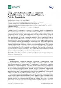
Figure 1: An LSTM network. The network has five input units, a hidden layer composed of two LSTM memory blocks and three output units. Each memory block has four inputs but only one output. All connections of the left block are drawn and other connections are skipped for simplicity.

ht = H(Wxh xt + Whh ht−1 + bh ) yt = Why ht + by where ht is the vector of hidden states, W denotes weight matrix connecting two layers (e.g. Wxh is the weights between input and hidden layer), b denotes bias vector (e.g. bh is the bias vector of hidden layer) and H is the activation function of hidden layer. Note that ht persists information from previous step’s hidden state ht−1 , and thus theoretically RNN can make use of all input history. However, in practice, the range of input history that can be accessed is limited, since the influence of a given input would decay or blow up exponentially as it circulates around the hidden states, which is known as vanishing gradient problem (Hochreiter et al., 2001). The most effective solution of this problem so far is the long short-term memory (LSTM) architecture (Hochreiter and Schmidhuber, 1997). An LSTM network is formed like the standard RNN except that the self-connected hidden units are replaced by special designed units called memory blocks as illustrated in Figure 1. The output of LSTM hidden layer ht given input xt is computed as following composite function (Graves et al., 2013): it = σ(Wxi xt + Whi ht−1 + Wci ct−1 + bi ) ft = σ(Wxf xt + Whf ht−1 + Wcf ct−1 + bf ) ct = ft ct−1 + it tanh(Wxc xt + Whc ht−1 + bc ) ot = σ(Wxo xt + Who ht−1 + Wco ct + bo ) ht = ot tanh(ct )

where σ is the logistic sigmoid function, and i, f , o and c are respectively the input gate, forget gate, output gate and cell activation vectors. Weights matrices are represented as arrows in Figure 1. These multiple gates allow the cell in LSTM memory block to store information over long periods of time, thereby avoiding the vanishing gradient problem. More interpretation about this architecture can be found in (Graves, 2012). Another shortcoming of conventional RNN is that only historic context can be exploited. In a typical tagging task where the whole sentence is given, it is helpful to exploit future context as well. Bidirectional RNN (BRNN) (Schuster and ...

yt−1

yt

yt+1

Backward Layer

← − h t−1

← − ht

← − h t+1

Forward Layer

→ − h t−1

→ − ht

→ − h t+1

xt−1

xt

xt+1

Outputs

Inputs

...

...

...

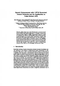
Figure 2: Bidirectional RNN Paliwal, 1997) offers an effective solution that can access both the preceding and succeeding contexts by involving two separate hidden layers. As illustrated in Figure 2, BRNN first computes the for→ − ward hidden sequence h and the backward hid← − den sequence h respectively, and then combines

− → ← − ht and ht to generate output yt . The process can be expressed as: → − − → →) →− → h t−1 + b− → xt + W − ht = H(Wx− h h h h ← − ← − − x + W← −) −← − h t+1 + b← ht = H(Wx← h h h h t ← − → − − h + by → h t + W← y t = W− hy t hy Replacing the hidden states in BRNN with LSTM memory blocks gives bidirectional LSTM (BLSTM) (Graves and Schmidhuber, 2005), i.e., the main architecture used in this paper, which can incorporate long periods of contextual information from both directions. Besides, as feedforward layers stacked in deep neural networks, the BLSTM layer can also be stacked on the top of the others to form a deep BLSTM architecture. As a type of RNN, deep BLSTM can be trained via various gradient-based algorithms designed for general RNN, for example, real-time recurrent learning (RTRL) and back-propagation through time (BPTT). In this work, we use the BPTT algorithm as described in (Graves, 2012) since it is conceptually simple and efficient for computation.

3 Tagging System The schematic diagram of BLSTM-RNN based tagging system is illustrated in Figure 3. Given sentence

. . . wn−1 , wn , wn+1 . . .

BLSTM-RNN tag probability distribution

. . . o(wn−1 ), o(wn ), o(wn+1 ) . . .

Decorder tags

′ ′ . . . yn−1 , yn′ , yn+1 ...

Figure 3: BLSTM-RNN based tagging system a sentence w1 , w2 , ..., wn with tags y1 , y2 , ..., yn , BLSTM-RNN is first used to predict the tag probability distribution o(wi ) of each word, then a decoding algorithm is proposed to generate the final predicted tags y1′ , y2′ , ..., yn′ . 3.1

BLSTM-RNN for tagging

The usage of BLSTM RNN is illustrated in Figure 4. Here wi is the one hot representation of the current word which is a binary vector with dimension |V | where V is the vocabulary. To reduce |V |,

o(wi )

output layer

BLSTM

hidden layer input layer

Ii W1

W2

wi

f (wi )

Figure 4: Usage of BLSTM-RNN for tagging each letter of input word is transferred to its lowercase. The upper case information is kept by introducing a three-dimensional binary vector f (wi ) to indicate if wi is full lowercase, full uppercase or leading with a capital letter. The input vector Ii of the network is computed as: Ii = W1 wi + W2 f (wi ) where W1 and W2 are weight matrixes connecting two layers. W1 wi is also known as the word embedding of wi which is a real-valued vector with a much smaller dimension than wi . In practice, to reduce the computational cost, W1 is implemented as a lookup table, W1 wi is returned by referring to wi ’s word embedding stored in this table. The output layer is a softmax layer whose dimension is the number of tag types. It outputs the tag probability distribution of word wi . 3.2 Decoding According to BLSTM-RNN, the obtained probability distribution of each step is supposed independent with each other. However, in some tasks such as NER and chunking, tags are highly related with each other and a few of types of tags can only follow specific types of tags. To make use of this kind of labeling constraints, we introduce a transition matrix A between each step’s output as illustrated in Figure 5. Each circle represents o(w1 )

o(w2 )

o(w2 )

.. .

.. .

.. .

...

o(wn )

t1 t2

...

.. .

tm A

A

Figure 5: Illustration of decoding. o(wi ) is the output of BLSTM-RNN, a probability distribution of m tag types.

a tag probability predicted by BLSTM-RNN, Aij stores the score of transition from tag ti to tj . The score is determined in a very simple way that if tj appears immediately behind ti in training corpus, Aij is 1, otherwise 0. It implies that tag bigrams that do not appear in training corpus are supposed invalid and would not appear in test case, no matter whether they are actually valid. The score of a sentence w1 , w2 , ..., wn ([w]n1 for short) along a path of tags y1 , y2 , ..., yn ([y]n1 for short) is then given by the product of transition score and BLSTMRNN output probability: s([w]n1 , [y]n1 )

n Y (Ayi−1 yi × o(wi )yi ) = i=1

The goal of decoding is to find the path which gives the highest sentence score: [y ′ ]n1 = arg max s([w]n1 , [y]n1 ) [y]n 1

This is a typical dynamic programming problem and can be solved with Viterbi algorithm (Viterbi, 1967).

4 Word Embedding As a neural network, BLSTM-RNN can easily adopt already trained word embedding by initializing W1 (illustrated in Figure 4) with those external embeddings. Currently, many word embeddings trained on very large corpora are available on line. However, these embeddings are trained by neural networks that are very different from BLSTM-RNN. This inconsistency is supposed as an shortcoming to make the most of these trained word embeddings. To conquer this shortcoming, we also propose a novel method to train word embedding on unlabeled data with BLSTM-RNN. In this method, BLSTM-RNN is applied to perform a tagging task with only two types of tags to predict: incorrect/correct. The input is a sequence of words which is a normal sentence with some words replaced by words randomly chosen from vocabulary. The words to be replaced are chosen randomly from the sentence. For those replaced words, their tags are 0 (incorrect) and for those that are not replaced, their tags are 1 (correct). A simple sample is shown in Figure 6. Although it is possible that some replaced words are also reasonable in the sentence, they are still considered “incorrect”. Then BLSTM-RNN is trained to minimize the binary classification error on the training

original sentence: They seem to be

prepared to

make . . .

input sentence: They beast to

be

austere

to

make . . .

tags: 0 1

1

0

1

1

1

...

Figure 6: Sample of constructed corpus for training word embedding. corpus. The neural network structure is the same as that in Figure 4. When the neural network is trained, W1 contains all trained word embeddings.

5 Experiments All of our approaches are implemented based on CURRENT (Weninger et al., 2014), an open source GPU-based toolkit of BLSTM-RNN. For constructing and training the neural network, we follow the default setup of CURRENT: The activation functions of input layer and hidden layers are logistic function, while the output layer uses softmax function for multiclassification. Neural network is trained using statistical gradient descent algorithm with constant learning rate. In all experiments, consecutive digits occurring within a word are relpaced with the symbol “#” . For example, both words “Tel192” and “Tel6” are converted into “Tel#”. The vocabulary we used is the most common 100,000 words in North American news corpus (Graff, 2008), plus one single “UNK” symbol for replacing all out of vocabulary words. 5.1 Tasks In this section, we briefly introduce three typical tagging tasks and their experimental setup on which we evaluate the performance of the proposed approach: part-of-speech tagging (POS), chunking (CHUNK) and named entity recognition (NER). POS is the task of labeling each word with its part of speech, e.g. noun, verb, adjective, etc. Our POS tagging experiment is conducted on the Wall Street Journal data from Penn Treebank III (Marcus et al., 1993). Training, development and test sets are split following setup in (Collins, 2002). Table 1 lists statistical information of the three data sets. Performance is evaluated by the accuracy of predicted tags on test set. CHUNK, also known as shallow parsing, divides a sentence into phrases that each phrase con-

Data Set Training Develop Test

WSJ sec. IDs Sentences# 0-18 38,219 19-21 5,527 22-24 5,462 # of tag types

Tokens# 912,344 131,768 129,654 45

Table 1: POS tagging corpus (WSJ in PTB III)

tains syntactically related words, such as noun phrase (NP), verb phrase (VP), etc. To identify the phrase boundaries, we use a commonly used IOBES tagging scheme that further fractionizes each tag type into four subtypes to indicate whether the word is inside (I), outside (O), begin (B), end(E) a multiple words chunk or a single word chunk (S). We conduct our experiment on a standard experimental setup of CHUNK according to the CoNLL-2000 shared task (Sang and Buchholz, 2000). Basic information about this setup is listed in Table 2. Performance is assessed by Data Set WSJ sec. IDs Sentences# Training 15-18 8,936 Develop N/A N/A Test 20 2,012 # of tag types (IOBES scheme)

Tokens# 211,727 N/A 47,377 42

Table 2: CHUNK corpus (WSJ in PTB III: CoNLL-2000) the F1 score computed by the evaluation script released by the CoNLL-2000 shared task1 . NER recognizes phrases of named entities such as names of persons, organizations and locations. IOBES tagging scheme is also applied in this task. Our experimental setup follows the CoNLL2003 shared task (Tjong Kim Sang and De Meulder, 2003). Table 3 shows its basic information. Performance is measured by the F1 score calcuData Set Sentences# Training 14,987 Develop 3,466 Test 3,684 # of tag types (IOBES scheme)

Tokens# 203,621 51,362 46,435 17

Table 3: NER corpus (CoNLL-2003) lated by the evaluation script of the CoNLL-2003 shared task 2 . 1 http://www.cnts.ua.ac.be/conll2000/ chunking 2 http://www.cnts.ua.ac.be/conll2003/ ner/

5.2 Network Structure In all experiments, without specific description, the input layer size is fixed to 100 and output layer size is set as the number of tag types according to the specific tagging task. In this experiment, we evaluate different sizes of hidden layer in BLSTM-RNN to pick up the best size for later experiments. Performances on three tasks are shown in Figure 7. It shows that

(a) POS

(b) CHUNK

(c) NER

Figure 7: Performance of BLSTM-RNN with different hidden layer sizes. Horizontal axis is the hidden layer size, vertical axis is respectively accuracy for POS, or F1 score for CHUNK and NER. hidden layer size has a limited impact on performance when it becomes large enough. To keep a good trade-off of accuracy, model size and training time, we choose 100 which is the smallest layer size to get a “reasonable” performance as the hidden layer size in all the following experiments. Besides, we also evaluate deep structure which uses multiple BLSTM layers. This deep BLSTM has been reported achieving significantly better performance than single layer BLSTM in various applications such as speech synthesis (Fan et al., 2014; Fernandez et al., 2014), speech recognition (Graves et al., 2013) and handwriting recognition (Graves and Schmidhuber, 2009). Table 4 compares the performance of BLSTM-RNNs with one (B) and two (BB) hidden layers. Size of all hidden layers is set 100. Using more layers brings a Sys B BB

POS(Acc) 96.60 96.63

CHUNK(F1) 91.91 91.76

NER(F1) 82.52 82.66

Table 4: Comparison of systems with one and two BLSTM hidden layers. slightly improvement for NER task, while does not show much help for POS and slightly decreases the performance of CHUNK. A possible explanation is that one BLSTM layer is adequate to learn an effective model for tasks like POS and CHUNK

Sys BLSTM BLSTM+Decoder

POS 96.60 96.60

CHUNK 90.60 91.71

NER 80.85 82.52

Table 6: Comparison of systems without and with decoder. which are relatively simple compared with NER or speech tasks, thus in these cases involving more layers would not provide a further help. Meanwhile additional more parameters makes the network harder to converge to a locally optimal model which leads to a worse performance. Based on this observation, in following experiments, BLSTMRNN is set only one hidden layer. 5.3

Decoder

In this experiment, we test the effect of decoder. Performance of BLSTM tagging systems without and with decoder are listed in Table 6. Without using decoder, predicted tag y ′ is determined by directly selecting the tag with the highest probability among network output o(wi ). The results show that decoder significantly improves the performance of CHUNK and NER tasks, though shows no help for POS. For this difference of improvment, we provide a possible explanation. In tasks like CHUNK and NER which uses IOBES tagging scheme, tags are highly dependent with their previous tags. For example, I-X can only appear behind B-X. CHUNK task has 42 tag types that can combine 42 × 42 = 1764 tag bigrams, but only 252 (14.3%) of them actually appear in training corpus. In NER task, 78 (27.0%) of total 289 tag bigrams have occurred more than once. Decoding in this case filters considerable invalid paths including more than half of candidates and thus improves the performance. As a contrast, in POS task, tags are directly predicted on each word without using any tagging schemes and thus do not have such strong dependence among tags. In POS training corpus, 1439 (71.0%) of total 2025 tag bigrams have occurred more than once. In this case, the dependences of tags are mainly learnt by BLSTM layer and the help from the decoder is very limited. The improvement provided by decoder shows that although BLSTM is considered can adopt contextual information automatically, the model is still far from ideal and a decoder with prior knowledge of tagging scheme is essential for achieving a good performance.

5.4 Word Embedding In this experiment, we evaluate BLSTM-RNN tagging approach using various of word embeddings including those trained by the proposed approach in Section 4 as well as four types of published word embeddings. To train word embeddings with our approach, we use North American news (Graff, 2008) as the unlabeled data. To construct corpus for training embeddings, the North American news data is first tokenized with the Penn Treebank tokenizer script 3 . Then about 20% words in normal sentences of the corpus are replaced with randomly selected word. BLSTM-RNN is trained to judge which word has been replaced as described in Section 4. To use word embedding, we just initialize the word embedding lookup table (W1 ) with these already trained embeddings. For words without corresponding external embeddings, their word embeddings are initialized with uniformly distributed random values, ranging from -0.1 to 0.1. Table 5 lists the basic information of involved word embeddings and performances of BLSTMRNN tagging approaches using these embeddings, where RCV1 represents the Reuters Corpus Volume 1 news set. RANDOM is the word embedding set composed of random values which is the baseline. BSLTMWE(10m), BSLTMWE(100m) and BSLTMWE(all) are word embeddings respectively trained by BLSTM-RNN on the first 10 million words, first 100 million words and all 536 million words of North American news corpus. While BSLTMWE(10m) does not bring about obvious improvement, BSLTMWE(100m) and BSLTMWE(all) significantly improve the performance. It shows that BLSTM-RNN can benefit from word embeddings trained by our approach and larger training corpus indeed leads to a better performance. This suggests that the result may be further improved by using even bigger unlabeled dataset. In our experiment, BSLTMWE(all) can be trained in about one day (23 hrs) on a NVIDIA Tesla M2090 GPU. The training time increases linearly with the training corpus size. When uses published word embeddings, the input layer size of BLSTM-RNN is set to the dimension of utiembeddings. All of the four published word embeddings significantly enhance BLSTMRNN. It proves that word embedding is a use3 https://www.cis.upenn.edu/˜treebank/ tokenization.html

WE

Dim

Vocab#

(Mikolov, 2010)

80

82K

(Collobert, 2011)

50

130K

(Mikolov et al., 2013b) (Pennington et al., 2014b) BLSTMWE(10m) BLSTMWE(100m) BLSTMWE(all) BLSTMWE(all) + (Collobert, 2011) RANDOM

300 100 100 100 100 100 100

3M 1193K 100K 100K 100K 113K 100K

Train Corpus (Toks #) Broadcast news (400M) RCV1+Wiki (221M+631M) Google news (10B) Twitter (27B) US news (10M) US news (100M) US news (536M) US news (536M) N/A

POS (Acc)

CHUNK (F1)

NER

96.97

92.53

84.69

97.02

93.76

89.34

96.85 97.02 96.61 97.10 97.26 97.26 96.61

92.45 93.01 91.91 93.86 94.44 94.59 91.71

85.80 87.33 84.66 86.47 88.38 89.64 82.52

Table 5: Comparison different word embeddings. System (Huang et al., 2012) (Toutanova et al., 2003) BLSTM

Acc 97.35 97.24 97.26

System (Sun et al., 2008) (Kudoh and Matsumoto, 2000) BLSTM

(a) POS

(b) CHUNK

F1 94.34 93.48 94.59

System (Ando and Zhang, 2005) (Florian et al., 2003) BLSTM

F1 89.31 88.76 89.64

(c) NER

Table 7: Top systems on three tagging tasks. State-of-the-art system is marked with bold type. ful feature and is an effective way to make use of big unlabeled data. Among all mentioned embeddings, BLSTMWE(all) achieves the best performance on POS and CHUNK tasks while slightly falls behind (Collobert, 2011) in NER task. One possible explanation is that (Collobert, 2011) is trained on Wikipedia data which contains more named entities, thereby their word embedding contains more useful information for NER task. BLSTMWE(all) is trained on a news corpus which is written with more formal grammar, thus it learns better representations for tagging syntactic role. Based on this conjecture, it is natural to expect the combination of (Collobert, 2011) and BLSTMWE(all) to bring a further improvement. This idea yields the BLSTMWE(all) + (Collobert, 2011). This word embeddings are first initialized with (Collobert, 2011) and then trained by BLSTM-RNN on North American corpus as BLSTMWE(all). This embeddings help BLSTM-RNN obtain the best performance in all three tasks. 5.5

Comparison with Previous Systems

In this section, we compare our approach with previous state-of-the-art systems on POS, CHUNK and NER tasks. Table 7 lists the related works of these three tasks. BLSTM represents the BLSTMRNN tagging approach using BLSTMWE(all) + (Collobert, 2011) word embeddings. POS: (Huang et al., 2012) reports the high-

est accuracy on WSJ test set (97.35%). Besides, (Moore, 2014) (97.34%) and (Shen et al., 2007) (97.33%) also reach accuracy above 97.3%. These three systems are considered as state-of-the-art systems in POS tagging. (Toutanova et al., 2003) is one of the most commonly used approaches which is also known as Stanford tagger. All of these methods utilize rich morphological features proposed in (Ratnaparkhi, 1996) which involves n-gram prefix and suffix (n = 1 to 4). Moreover, (Shen et al., 2007) also involves prefix and suffix of length from 5 to 9. (Moore, 2014) adds extra elaborately designed features, including flags indicating if word ends with −ed or −ing, etc. CHUNK: (Kudoh and Matsumoto, 2000) (93.48%) is the system ranked first in CoNLL2000 shared task challenge. Later, (Sun et al., 2008) reports the state-of-the-art F1 score (94.34%) on CoNLL-2000 task. Besides, (Sha and Pereira, 2003) (94.29%) and (McDonald et al., 2005) (94.29%) both report F1 score around 94.3%. These systems use features composing of words and POS tags. NER: (Florian et al., 2003) (88.76%) is the top system in CoNLL-2003 shared task challenge. (Ando and Zhang, 2005) (89.31%) reports a better F1 score with a semi-supervised approach. The unlabeled corpus they used is 27M words from Reuters. Features used in these works include words, POS tags, CHUNK tags, prefixes, suffixes, and a large gazetteer (geographical dictionary).

All of these top systems use rich features and feature sets in different tasks are quite different. In contrast, our system only uses one set of taskindependent features in all tasks and do not require any feature engineering to achieve the state-of-theart performance in CHUNK and NER tasks. In POS, our approach also get a competitive performance that is comparable with Stanford POS tagger. Our results show that feature engineering in conventional methods can be effectively replaced by built-in modeling of BLSTM-RNN.

6 Related Works (Collobert et al., 2011) is the most similar work as ours. It is a unified tagging solution based on neural network which also uses simple taskindependent features and word embeddings learnt from unlabeled text. The main difference is that (Collobert et al., 2011) uses feedforward neural network instead of BLSTM-RNN. A comparison of (Collobert et al., 2011) and our approach is listed in Table 8, where NN is the uniSys NN NN+WE BLSTM BLSTM+BLSTMWE

POS 96.37 97.20 96.61 97.26

CHUNK 90.33 93.63 91.71 94.59

NER 81.47 88.67 82.52 89.64

Table 8: Comparison of (Collobert et al., 2011) and our approach. fied tagging system of (Collobert et al., 2011) and NN+WE is that system using word embedding trained by their approach. Without using word embedding, BLSTM outperforms NN in all three tasks. It is consistent with the observations in previous works that BLSTM-RNN is a more powerful model for sequential labeling than feedforward network. With word embeddings, our approach also significantly surpasses NN+WE in all three tasks. (Suzuki and Isozaki, 2008) proposes a semisupervised approach which incorporates one billion words of unlabeled data during training. They claim that their model can be applied to various tasks and report the state-of-the-art performance on all these three tasks (97.40 for POS, 95.15 for CHUNK, 89.92 for NER). However, they also utilize rich feature templates for each task (47 feature templates for POS, 39 templates for CHUNK, 79 templates for NER) which makes their system not so unified. Their method still requires prior

knowledge to design these feature templates which limits its application to tasks that lack of knowledge or tools to extract necessary features. Besides, they have to train model with quite big unlabeled data for each task which would lead to a time consuming training process. In contrast, our approach separates the lengthy training for word embedding from the relatively fast training for the supervised tagging task. Once our word embeddings are trained, they can be regarded as a kind of linguistic resources like semantic dictionary and be directly used.

7 Conclusions In this paper, we propose a unified tagging solution based on BLSTM-RNN. This system avoids involving task-specific features, instead it utilizes word embeddings learnt automatically from unlabeled text. Without reliance on feature engineering or prior knowledge, this approach can be easily applied to various tagging tasks. Experiments are conducted on three typical tagging tasks: POS tagging, chunking and named entity recognition. Using simple task-independent input features, our approach gets nearly state-of-the-art results on all these three tasks. Our results suggest that BLSTM-RNN with word embedding is an effective unified tagging solution and worth further exploration.

References Rie Kubota Ando and Tong Zhang. 2005. A framework for learning predictive structures from multiple tasks and unlabeled data. The Journal of Machine Learning Research, 6:1817–1853. Yoshua Bengio, Holger Schwenk, Jean-S´ebastien Sen´ecal, Fr´ederic Morin, and Jean-Luc Gauvain. 2006. Neural probabilistic language models. In Innovations in Machine Learning, pages 137–186. Springer. Michael Collins. 2002. Discriminative Training Methods for Hidden Markov Models: Theory and Experiments with Perceptron Algorithms. In Proceedings of EMNLP, pages 1–8, Stroudsburg, PA, USA. Ronan Collobert and Jason Weston. 2008. A unified architecture for natural language processing: Deep neural networks with multitask learning. In Proceedings of the 25th International Conference on Machine learning, pages 160–167, Helsinki, Finland. Ronan Collobert, Jason Weston, L´eon Bottou, Michael Karlen, Koray Kavukcuoglu, and Pavel Kuksa.

2011. Natural Language Processing (almost) from scratch. The Journal of Machine Learning Research, 12:2493–2537. Ronan Collobert. 2011. SENNA. nec-labs.com/senna/.

Mitchell P Marcus, Mary Ann Marcinkiewicz, and Beatrice Santorini. 1993. Building a large annotated corpus of English: The Penn Treebank. Computational linguistics, 19(2):313–330.

http://ml.

Yuchen Fan, Yao Qian, Fenglong Xie, and Frank K. Soong. 2014. TTS synthesis with bidirectional LSTM based recurrent neural networks. In Proceedings of INTERSPEECH, Singapore.

Ryan McDonald, Koby Crammer, and Fernando Pereira. 2005. Flexible text segmentation with structured multilabel classification. In Proceedings of EMNLP, pages 987–994, Vancouver, British Columbia, Canada. Association for Computational Linguistics.

Raul Fernandez, Asaf Rendel, Bhuvana Ramabhadran, and Ron Hoory. 2014. Prosody contour prediction with long short-term memory, bi-directional, deep recurrent neural networks. In Proceedings of INTERSPEECH, Singapore.

Gr´egoire Mesnil, Xiaodong He, Li Deng, and Yoshua Bengio. 2013. Investigation of recurrent-neuralnetwork architectures and learning methods for spoken language understanding. In Proceedings of INTERSPEECH, pages 3771–3775, Lyon, France.

Radu Florian, Abe Ittycheriah, Hongyan Jing, and Tong Zhang. 2003. Named entity recognition through classifier combination. In Proceedings of CoNLL, pages 168–171, Edmonton, Canada.

Tomas Mikolov, Martin Karafi´at, Lukas Burget, Jan Cernock´y, and Sanjeev Khudanpur. 2010. Recurrent neural network based language model. In Proceedings of INTERSPEECH, pages 1045–1048, Makuhari, Chiba, Japan.

David Graff. 2008. North American News Text, Complete LDC2008T15. https://catalog.ldc. upenn.edu/LDC2008T15. Alex Graves and J¨urgen Schmidhuber. 2005. Framewise phoneme classification with bidirectional lstm and other neural network architectures. Neural Networks, 18(5):602–610. Alex Graves and J¨urgen Schmidhuber. 2009. Offline Handwriting Recognition with Multidimensional Recurrent Neural Networks. In Advances in Neural Information Processing Systems 21, pages 545–552. NIPS. Alex Graves, Abdel-rahman Mohamed, and Geoffrey Hinton. 2013. Speech recognition with deep recurrent neural networks. In Proceedings of ICASSP, pages 6645–6649, Vancouver, BC, Canada. Alex Graves. 2012. Supervised sequence labelling with recurrent neural networks, volume 385. Springer. Sepp Hochreiter and J¨urgen Schmidhuber. 1997. Long short-term memory. Neural computation, 9(8):1735–1780. Sepp Hochreiter, Yoshua Bengio, Paolo Frasconi, and J¨urgen Schmidhuber. 2001. Gradient flow in recurrent nets: the difficulty of learning long-term dependencies. Liang Huang, Suphan Fayong, and Yang Guo. 2012. Structured Perceptron with Inexact Search. In Proceedings of HLT-NAACL, pages 142–151, Montr´eal, Canada. Taku Kudoh and Yuji Matsumoto. 2000. Use of support vector learning for chunk identification. In Proceedings of CoNLL, pages 142–144, Lisbon, Portugal.

Tomas Mikolov, Kai Chen, Greg Corrado, and Jeffrey Dean. 2013a. Efficient estimation of word representations in vector space. In Proceedings of ICLR. Tomas Mikolov, Kai Chen, Greg Corrado, and Jeffrey Dean. 2013b. word2vec. https://code. google.com/p/word2vec/. Tomas Mikolov. 2010. RNNLM. http://rnnlm. org/. Robert Moore. 2014. Fast high-accuracy part-ofspeech tagging by independent classifiers. In Proceedings of Coling, pages 1165–1176, Dublin, Ireland. Jeffrey Pennington, Richard Socher, and Christopher Manning. 2014a. Glove: Global Vectors for Word Representation. In Proceedings of EMNLP, pages 1532–1543, Doha, Qatar. Jeffrey Pennington, Richard Socher, and Christopher D. Manning. 2014b. GloVe. http://nlp. stanford.edu/projects/glove/. Adwait Ratnaparkhi. 1996. A Maximum Entropy Model for Part-Of-Speech Tagging. In Proceedings of EMNLP, pages 133–142, Philadelphia, PA, USA. Erik F. Tjong Kim Sang and Sabine Buchholz. 2000. Introduction to the conll-2000 shared task chunking. In Proceedings of CoNLL, pages 127–132, Lisbon, Portugal. Mike Schuster and Kuldip K Paliwal. 1997. Bidirectional recurrent neural networks. Signal Processing, IEEE Transactions on, 45(11):2673–2681. Fei Sha and Fernando Pereira. 2003. Shallow parsing with conditional random fields. In Proceedings of HLT-NAACL, pages 134–141, Edmonton, Canada.

Libin Shen, Giorgio Satta, and Aravind Joshi. 2007. Guided Learning for Bidirectional Sequence Classification. In Proceedings of ACL, pages 760–767, Prague, Czech Republic. Xu Sun, Louis-Philippe Morency, Daisuke Okanohara, Yoshimasa Tsuruoka, and Jun’ichi Tsujii. 2008. Modeling latent-dynamic in shallow parsing: A latent conditional model with imrpoved inference. In Proceedings of Coling, pages 841–848, Manchester, UK. Coling 2008 Organizing Committee. Martin Sundermeyer, Ralf Schl¨uter, and Hermann Ney. 2012. LSTM Neural Networks for Language Modeling. In Proceedings of INTERSPEECH, Portland, Oregon, USA. Martin Sundermeyer, Tamer Alkhouli, Joern Wuebker, and Hermann Ney. 2014. Translation Modeling with Bidirectional Recurrent Neural Networks. In Proceedings of EMNLP, pages 14–25, Doha, Qatar. Martin Sundermeyer, Hermann Ney, and Ralf Schluter. 2015. From feedforward to recurrent lstm neural networks for language modeling. Audio, Speech, and Language Processing, IEEE/ACM Transactions on, 23(3):517–529. Jun Suzuki and Hideki Isozaki. 2008. Semi-supervised sequential labeling and segmentation using gigaword scale unlabeled data. In Proceedings of ACL, pages 665–673, Columbus, Ohio. Association for Computational Linguistics. Erik F Tjong Kim Sang and Fien De Meulder. 2003. Introduction to the conll-2003 shared task: Language-independent named entity recognition. In Proceedings of CoNLL, pages 142–147, Edmonton, Canada. Association for Computational Linguistics. Kristina Toutanova, Dan Klein, Christopher D. Manning, and Yoram Singer. 2003. Feature-Rich Partof-Speech Tagging with a Cyclic Dependency Network. In Proceedings of HLT-NAACL, pages 173– 180, Edmonton, Canada. Joseph Turian, Lev Ratinov, and Yoshua Bengio. 2010. Word Representations: A Simple and General Method for Semi-supervised Learning. In Proceedings of ACL, pages 384–394, Stroudsburg, PA, USA. Andrew.J. Viterbi. 1967. Error bounds for convolutional codes and an asymptotically optimum decoding algorithm. Information Theory, IEEE Transactions on, 13(2):260–269. Felix Weninger, Johannes Bergmann, and Bj¨orn Schuller. 2014. Introducing CURRENNT–the Munich open-source CUDA RecurREnt Neural Network Toolkit. Journal of Machine Learning Research, 15. Kaisheng Yao, Geoffrey Zweig, Mei-Yuh Hwang, Yangyang Shi, and Dong Yu. 2013. Recurrent neural networks for language understanding. In

Proceedings of INTERSPEECH, pages 2524–2528, Lyon, France.