Bilinear Transformations via a Computer Algebra System - ATCM

Bilinear Transformations via a Computer Algebra System Tilak de Alwis [email protected] Department of Mathematics Southeastern Louisiana University Hammond, LA 70403 USA Abstract: In this paper, we will investigate several properties of bilinear transformations using a computer algebra system. Bilinear transformations, also known as linear fractional transformations or Möbius transformations belong to a wider class of functions known as conformal mappings in complex analysis. It is well-known that bilinear transformations carry a circle or a straight line in one complex plane to a circle or a straight line in another complex plane. Due to the graphical nature of these transformations, a computer algebra system such as Mathematica is an ideal tool to further study their properties. In the process we will observe several new non-standard results, which can be proved using traditional methods without resorting to any computer algebra system. The paper uses Mathematica version 7.0 on a Windows XP platform, but identical results can be obtained by using any other computer algebra system of reader’s choice.

1. Introduction A bilinear transformation in complex analysis is a mapping f defined by the following formula, where a, b, c, and d are complex numbers with ad − bc ≠ 0 (see [1], [2], and [6]).

f ( z) =

az + b cz + d

(1.1)

For simplicity, in the paper, we will restrict a, b, c, and d to be real numbers, even though a similar analysis can be carried out for the general case. The above map carries in general, a complex number z = x + iy in the XY-plane to another complex number w = u + iv in the UV-plane. In the traditional definition of a bilinear transformation, as stated above, one would normally assume that ad − bc ≠ 0 . The reason behind this assumption is that if ad − bc = 0 , a mapping of the kind defined by equation (1.1) is not interesting: In that case, as the following discussion shows, f maps the entire complex plane, except perhaps a single point into a fixed point in another complex plane, i.e. f would become a constant map: Suppose ad − bc = 0 . We will still assume that (c, d ) ≠ (0,0) , as otherwise f is not well-defined. The argument can be divided into several cases:

Case 1: c ≠ 0 and d ≠ 0 In this case, since ad − bc = 0 , one can write a / c = b / d = k for some real constant k. Then it follows that f ( z ) = (ckz + dk ) /(cz + d ) = k , provided that z ≠ − d / c . In other words, in the present

case, f maps the entire complex plane, except the point z = − d / c into a single point in another complex plane. Case 2: c = 0 and d ≠ 0 In this case it easily follows that a = 0 , and thus f ( z ) = b / d . Therefore, in this case f maps the entire complex plane into a single point in another complex plane. Case 3: c ≠ 0 and d = 0 In this case it easily follows that b = 0 , and thus f ( z ) = az /(cz ) = a / c , provided that z ≠ 0 . In other words, f maps the entire complex plane minus the origin into a single point in another complex plane. Thus, the case ad − bc = 0 is not interesting and that is why we assume that ad − bc ≠ 0 in the traditional definition of a bilinear transformation. A well-known theorem in complex analysis states that such a transformation carries a circle or a straight line in one complex plane to a circle or a straight line in another complex plane (see [1], [2], and [6]). The paper focuses on this result, but first it will be a good idea to find out exactly under what conditions circles are mapped into circles, circles are mapped into straight lines, straight lines are mapped into circles, and straight lines are mapped into straight lines. Thus, in the next sections of the paper, we will analyze the proof of this theorem carefully. We will also use the programming capabilities of the computer algebra system (CAS) Mathematica to visualize how circles are mapped to straight lines etc. Mathematica is a general purpose CAS and has its own powerful programming language (see [4] and [5]). Combining this programming language with built in graphics capabilities, one can use Mathematica as an excellent visualization tool. Such visualization powers facilitated by modern technologies can unveil an abundance of interesting results or questions that are not usually discussed in the traditional literature on bilinear transformations: For example, if f caries a straight line l 1 into another straight line l 2 , then under what conditions these two lines are parallel, or perpendicular? Likewise, assuming f carries a circle C1 into another circle C 2 , then under what conditions one circle touches the other, internally or externally? Another interesting question is to ask under what conditions the circle C1 will be identical to the circle C 2 without f being the identity map. An integral part of this paper is to answer such questions. The paper also motivates the inquisitive reader to pose his own questions on bilinear transformations via experimentations with a computer algebra system, to form conjectures, and then to prove them mathematically.

2. The Image of a Circle under a Bilinear Transformation In this section, we will consider the image of a circle C centered at the origin, in the XY-plane under the bilinear transformation defined by equation (1.1). One can write the equation of the circle C in the following form where r is its radius: x2 + y2 = r 2

(2.1)

Let z = x + iy represent any point on the circle given by equation (2.1), which means that | z |= r . Let w = u + iv where u, v ∈  be the image of z under the bilinear transformation f given by equation (1.1). Thus, we have the following relationship: w = u + iv = f ( z ) =

az + b cz + d

(2.2)

At this point, it is fine to assume that z is such that cz + d ≠ 0 , so that the equation (2.2) is welldefined. It is not too difficult to show that the condition d 2 − c 2 r 2 ≠ 0 is equivalent to the fact that there is no complex number z1 = x1 + iy1 on the circle (2.1) such that cz1 + d = 0 . We will very soon see the significance of this condition. The equation (2.2) implies that z (a − cw) = dw − b . Taking the modulus of both sides and noting that | z | = r , and w = u + iv , one obtains the following: | (b − du ) − idv | = r | (a − cu ) − icv |

(2.3)

The above equation (2.3) implies that (b − du ) 2 + d 2 v 2 = r 2 [(a − cu ) 2 + c 2 v 2 ] , which is equivalent to the following key equation: u 2 (d 2 − c 2 r 2 ) + v 2 (d 2 − c 2 r 2 ) + 2u (acr 2 − bd ) + b 2 − r 2 a 2 = 0

(2.4)

In order to see why does the equation (2.4) represent a circle or a straight line, one has to consider the following two cases: Case 1: d 2 − c 2 r 2 ≠ 0 By completing the squares on the left-hand side, one can easily show that equation (2.4) represents a circle with the following information (see [3]): Center = ( − (acr 2 − bd ) /(d 2 − c 2 r 2 ), 0 )

(2.5)

Radius = r | ad − bc | / | d 2 − c 2 r 2 |

(2.6)

Case 2: d 2 − c 2 r 2 = 0 Note that this condition guarantees that acr 2 − bd ≠ 0 : We would leave the reader to verify that if both d 2 − c 2 r 2 = 0 and acr 2 − bd = 0 , that would imply ad − bc = 0 , contradicting one of initial assumptions in the introduction (see the paragraph before equation (1.1)). Therefore, in this case the equation (2.4) represents a vertical line in the UV-plane whose equation is given by u = (r 2 a 2 − b 2 ) /[2(acr 2 − bd )]

(2.7)

By the remarks just following equation (2.2), the condition d 2 − c 2 r 2 = 0 guarantees that there is a point z1 = x1 + iy1 on the circle C such that cz1+d = 0 . The bilinear transformation f carries this point z1 to the point at infinity in the UV-plane, while all other points of the circle C are carried into the vertical line given by equation (2.7). In other words, the condition d 2 − c 2 r 2 = 0 is exactly what enables the circle C, a closed curve to be mapped into a straight line, a non-closed curve.

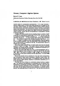
A CAS such as Mathematica enables one to visualize how a circle can be mapped into another circle or a straight line. In our first Program 2.1, one can choose the input values a, b, c, d, and r such that ad − bc ≠ 0 and d 2 − c 2 r 2 ≠ 0 . As described in case 1 previously, the condition d 2 − c 2 r 2 ≠ 0 ensures that the circle C will be mapped into another circle. The program plots the source circle C in dashed blue, and the image circle given by equation (2.4) in solid red, in the same coordinate plane. Program 2.1 f[z_] := (a*z + b)/(c*z + d); g[x_, y_] := x^2 + y^2 - r^2; (* Pick a,b,c,d, and r manually such that a*d-b*c is nonzero and d^2-r^2*c^2 is nonzero *) a = 1; b = 2; c = 1; d = 3; r = 1; x1[t_]:= r*Cos[t]; y1[t_]:= r*Sin[t]; x2[t_]:= Simplify[Re[Expand[f[x1[t] + I*y1[t]]]], Assumptions-> t∈Reals] y2[t_]:= Simplify[Im[Expand[f[x1[t] + I*y1[t]]]], Assumptions-> t∈Reals] p1 = ParametricPlot[{x1[t], y1[t]}, {t, 0, 2 Pi}, PlotStyle -> {RGBColor[0, 0, 1], Dashing[{0.02,0.02}]}]; p2 = ParametricPlot[{x2[t], y2[t]}, {t, -10, 10}, PlotRange -> {{-1.5, 1.5}, {-1.5, 1.5}}, PlotStyle -> {Thickness[1/150], RGBColor[1, 0, 0]}]; Show[{p1, p2}, PlotRange -> {{-1.5, 1.5}, {-1.5, 1.5}}, AspectRatio -> Automatic]

In order to execute the program, place the cursor on anyone of the program lines and press “ShiftEnter” (see [4] and [5]). The output is given below: 1.5

1.0

0.5

- 1.5

- 1.0

- 0.5

0.5

1.0

1.5

- 0.5

- 1.0

- 1.5

Figure 2.1 The source circle (dashed line) is mapped to the image circle (solid line), where a = 1, b = 2, c = 1, d = 3, and r = 1

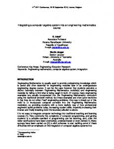
The Program 2.1 is quite useful in the sense that by changing the input values for a, b, c, d, and r, the user can experiment with different types of bilinear transformations. For example, one might be curious as to when would the image circle be also centered at the origin. As implied by equation (2.5), the additional condition is precisely acr 2 − bd = 0 . For example, for the choice of a = 4, b = 2, c = 1, d = 2, and r = 1 , we have all the conditions ad − bc ≠ 0, d 2 − c 2 r 2 ≠ 0, and

acr 2 − bd = 0 . Therefore, the corresponding bilinear transformation maps the source circle | z | = 1 to another circle centered at the origin, as shown in the diagram below: 2

1

-2

-1

1

2

-1

-2

Figure 2.2 The source circle | z | = 1 (dashed line) is mapped to the image circle (solid line) centered at the origin, where a = 4, b = 2, c = 1, d = 2, and r = 1

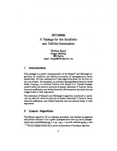
We were experimenting with different values for a, b, c, d, and r, and accidentally noticed that for a = 4, b = −1, c = 1, d = 2, and r = 1 , the source circle touches the image circle internally, as shown below: 3

2

1

-4

-2

2 -1

-2

-3

-4

Figure 2.3 The source circle | z | = 1 (dashed line) touches the image circle (solid line), where a = 4, b = −1, c = 1, d = 2, and r = 1

The motivation for the following theorem was provided by the above observation. Theorem 2.1 Consider the bilinear transformation given by f ( z ) = (az + b) /(cz + d ) where a, b, c,

d, are real numbers such that ad − bc ≠ 0 . Let C be the circle given by | z | = r where r > 0 is such

that d 2 − c 2 r 2 ≠ 0 , which ensures that the image of C under f is another circle $ ' . Then a necessary and sufficient condition for these two circles to touch is given by | acr 2 − bd | = r | | ad − bc | ± | d 2 − c 2 r 2 | | The “+” sign in the above corresponds to the external touching of the circles, and the “ -”sign to internal touching. Proof. Since the centers of both circles are on the x-axis, a necessary and sufficient condition for their touching is that the distance between their centers is equal to | r ± r ' | where r ' is the radius of the image circle $ ' . Now use the equations (2.5) and (2.6), and the details are left to the reader. ■

Going back to case 2, where d 2 − c 2 r 2 = 0 (just below equation (2.6)), we noticed that in this case f maps a circle into a straight line. The following program illustrates this case:

Program 2.2 f[z_]:=(a*z+b)/(c*z+d); g[x_,y_]:=x^2+y^2-r^2; (*Pick a,b,c,d,and r manually such that a*d-b*c is nonzero and d^2-r^2*c^2 is zero*) a=1; b=2; c=4; d=4; r=1; x1[t_]:=r*Cos[t]; y1[t_]:=r*Sin[t]; x2[t_]:=Simplify[Re[Expand[f[x1[t]+I*y1[t]]]], Assumptions->t∈Reals] y2[t_]:=Simplify[Im[Expand[f[x1[t]+I*y1[t]]]], Assumptions->t∈Reals] p1=ParametricPlot[{x1[t],y1[t]},{t,0,2Pi}, PlotStyle->{RGBColor[0,0,1],Dashing[{0.02,0.02}]}]; p2=ParametricPlot[{x2[t],y2[t]},{t,-10,10},PlotPoints->100, PlotStyle->{Thickness[1/150],RGBColor[1,0,0]}]; Show[{p1,p2},PlotRange->{{-2,2},{-2,2}},AspectRatio->Automatic]

The output of the program is given below: 2

1

-2

-1

1

2

-1

-2

Figure 2.4 The source circle | z | = 1 (dashed line) is mapped to a straight line (solid line), where a = 1, b = 2, c = 4, d = 4, and r = 1

3. The Image of a Straight Line Under a Bilinear Transformation In this section we will investigate the image of a straight line l in the XY-plane under the bilinear transformation given by equation (1.1). One can write the equation of l as follows, where p, q, and r are real numbers with ( p, q) ≠ (0, 0) : px + qy + r = 0 (3.1) Let z = x + iy where x, y ∈  be any point on the line l . Let w = u + iv where u, v ∈  be the image of z under f, which means that w = (az + b) /(cz + d ) . This implies that z = (b − wd ) /( wc − a) , or the following equivalent form: b − d (u + iv) (3.2) x + iy = c(u + iv) − a By matching the real parts of both sides, and also the imaginary parts of both sides of equation (3.2) one obtains the following (see [6]):

x =

u (ad + bc) − ab − cd (u 2 + v 2 ) (cu − a ) 2 + c 2 v 2

y=

v(ad − bc) (cu − a) 2 + c 2 v 2

(3.3)

However, x and y given above must satisfy the equation (3.1). Therefore, by substituting and simplifying, one obtains the following relationship between u and v: (u 2 + v 2 )(rc 2 − pcd ) + u[ p(ad + bc) − 2acr ] + qv(ad − bc) + a 2 r − pab = 0

(3.4)

The above equation (3.4) represents the image in the UV-plane of the straight line px + qy + r = 0 under the bilinear transformation f. We will now consider two cases: Case 1: rc 2 − pcd ≠ 0 In this case, the equation (3.4) represents a circle in the UV-plane. By completing the square, one can obtain the center and the radius of this circle (see [3]):  ( pbc + pad − 2acr ) q (ad − bc)   Center =  , 2c( pd − rc) 2c( pd − rc)  

Radius =

1 2

p2 + q2

ad − bc c( pd − rc)

(3.5)

(3.6)

Case 2: rc 2 − pcd = 0 In this case, (3.4) represents a straight line in the UV-plane, whose equation is given by u[ p(ad + bc) − 2acr ] + qv(ad − bc) + a 2 r − pab = 0

(3.7)

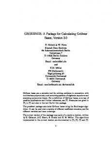
One can write a Mathematica program similar to Program 2.1 or 2.2 to visualize the image of a straight line under a bilinear transformation. The following Program 3.1 maps a straight line to a circle by choosing a, b, c, d, p, q, and r such that above case 1 is satisfied: Program 3.1 f[z_]:=(a*z+b)/(c*z+d); g[x_,y_]:=p*x+q*y+r; (*Pick a,b,c,d and p,q,r manually such that a*d-b*c is nonzero and r*c^2-p*c*d is nonzero*) a=1; b=2; c=1; d=6; p=1; q=1; r=-3; x1[t_]:=If[q!=0,t,-r/p]; y1[t_]:=If[q!=0,-(r+p*t)/q,t]; x2[t_]:=Simplify[Re[Expand[f[x1[t]+I*y1[t]]]], Assumptions->t∈Reals] y2[t_]:=Simplify[Im[Expand[f[x1[t]+I*y1[t]]]], Assumptions->t∈Reals] p1=ParametricPlot[{x1[t],y1[t]},{t,-10,10}, PlotStyle->{RGBColor[0,0,1], Dashing[{0.02,0.02}]}]; p2=ParametricPlot[{x2[t],y2[t]},{t,-50,50}, PlotPoints->200, PlotStyle->{Thickness[1/150], RGBColor[1,0,0]}]; Show[{p1,p2}, PlotRange->{{-2,4},{-1,4}}, AspectRatio->Automatic]

The output of the program is given below: 4

3

2

1

-2

-1

1

2

3

4

-1

Figure 3.1 The source straight line px + qy + r = 0 (dashed line) is mapped to a circle (solid line), where a = 1, b = 2, c = 1, d = 6 and p = 1, q = 1, r = −3

On the other hand, if we choose a = −2, b = 2, c = 2, d = 3 and p = 2, q = 1, r = 3 , the conditions ad − bc ≠ 0 and rc 2 − pcd = 0 are satisfied, mapping a straight line into another straight line, as mentioned in case 2. See the diagram below: 2

1

-2

-1

1

2

-1

-2

Figure 3.2 The source straight line px + qy + r = 0 (dashed line) is mapped to another straight line (solid line), where a = −2, b = 2, c = 2, d = 3 and p = 2, q = 1, r = 3

The situation given in above Figure 3.2 made us curious to investigate when the source straight line will be perpendicular to the image straight line. In the process, the following theorem was discovered: Theorem 3.1 Consider the bilinear transformation given by f ( z ) = (az + b) /(cz + d ) where a, b, c, d, are real numbers such that ad − bc ≠ 0 . Let l be the straight line given by px + qy + r = 0 where

p, q, and r are real numbers with ( p, q ) ≠ (0, 0) . Suppose further that rc 2 − pcd = 0 , which ensures

that the image of l under f is another straight line l' . (a) A necessary and sufficient condition for l and l' to be perpendicular is c ≠ 0 and p = ± q . (b) A necessary and sufficient condition for l and l' to be parallel is pq = 0 or c = 0 . Proof. (a) It is clear that two straight lines a1 x + b1 y + c1 = 0 and a2 x + b2 y + c2 = 0 are perpendicular if and only if a1b1 + a2b2 = 0 . Since l and l' are given by equations (3.1) and (3.7) respectively, using the fact just mentioned, a necessary and sufficient condition for perpendicularity is the following:

p ( pbc + pad − 2acr ) + q 2 (ad − bc) = 0 ⇔ p 2 (ad + bc) − 2acpr + q 2 (ad − bc) = 0 ⇔ (c ≠ 0 and p 2 (ad + bc) − 2acpr + q 2 (ad − bc) = 0) or (c = 0 and p 2 (ad + bc) − 2acpr + q 2 (ad − bc) = 0) ⇔ (c ≠ 0 and p 2 (ad + bc) − 2acp( pd / c) + q 2 (ad − bc) = 0) or (c = 0 and p 2 (ad + bc) − 2acpr + q 2 (ad − bc) = 0) ⇔ ⇔ ⇔ ⇔

( ( ( (

c≠0 c≠0 c≠0 c≠0

and and and and

( p 2 − q 2 )(ad − bc) = 0 ) or ( c = 0 and ad ( p 2 + q 2 ) = 0 ) p = ± q ) or ( c = 0 and ad = 0 ) p = ± q ) or ( c = 0 and a = 0 ) or ( c = 0 and d = 0 ) p = ±q )

(b) Use the fact that two straight lines a1 x + b1 y + c1 = 0 and a2 x + b2 y + c2 = 0 are parallel if and only if a1b2 − a2b1 = 0 . The details are left to the reader. ■ We can also use Mathematica to support the accuracy of the above Theorem 3.1. The following program performs this task for part (a) of the theorem. Program 3.3 f[z_]:=(a*z+b)/(c*z+d); g[x_,y_]:=p*x+q*y+r; a=RandomReal[{1,100}]; b=RandomReal[{1,100}]; c=RandomReal[{1,100}]; (* With this choice, c becomes nonzero *) d=RandomReal[{b*c/a+1,b*c/a+100}]; (*With this choice of d, ad-bc becomes nonzero*) p=RandomReal[{1,100}]; q=RandomChoice[{-1,1},1][[1]]*p; (*This randomly chooses q to be either p or -p *) r=p*d/c; (* With this choice, r*c^2-p*c*d is zero*) x1[t_]:=If[q!=0,t,-r/p]; y1[t_]:=If[q!=0,-(r+p*t)/q,t]; x2[t_]:=Simplify[Re[Expand[f[x1[t]+I*y1[t]]]], Assumptions->t∈Reals] y2[t_]:=Simplify[Im[Expand[f[x1[t]+I*y1[t]]]], Assumptions->t∈Reals] p1=ParametricPlot[{x1[t],y1[t]},{t,-15,15}, PlotStyle->{RGBColor[0,0,1], Dashing[{0.02,0.02}]}]; p2=ParametricPlot[{x2[t],y2[t]},{t,-500,500}, PlotPoints->200, PlotStyle->{Thickness[1/150], RGBColor[1,0,0]}]; Show[{p1,p2}, AspectRatio->Automatic, Axes->True]

The program picks a, b, c as random real numbers from 1 to 100. Among other things, this ensures c is non zero. Since the program chooses d as a random real number between (bc / a) + 1 , and (bc / a ) + 100 , d cannot be equal to (bc / a ) , meaning that ad − bc will be nonzero. The program also chooses p as any random real number between 1 and 100, and q is randomly chosen to be either p or − p . Since r is defined as pd / c , the condition rc 2 − pcd = 0 is also satisfied. Thus all the requirements of Theorem 3.1(a) are satisfied, and each time the program is executed, one can observe that the image straight line is perpendicular to the source straight line. However, the user is warned that sometimes not both lines might be visible in the output – if that happens the

“PlotRange” command of Mathematica can be used to define a new graphing window (see [5]). The biggest advantage of the above program is that the user does not have to manually input values for a, b, c, d, p, q, etc.

Conclusion In this paper, we showed how to use a CAS to make further investigations on bilinear transformations. In the process several non standard results were discovered. Modern technologies such as CAS can certainly shed new light into traditional mathematics topics, giving them more life and new meaning. Following the spirit of the paper, the reader is encouraged to carry out more experiments to discover further results on these transformations – the amount of discoveries that can be made is only limited by his or her imagination! References

[1] [2] [3] [4]

Ahlfors, Lars. (1979). Complex Analysis. New York, NY: McGraw-Hill Bak, J. and Newman D. J. (1982). Complex Analysis. New York, NY: Springer-Verlag Dugopolski, M. (2003). College Algebra. Boston, MA: Addison-Wesley/Pearson Gray, T. and Glynn, J. (2000). The Beginner’s Guide to Mathematica, Version 4. Cambridge, UK: Cambridge University Press. [5] Wolfram, S. (2003). Mathematica Book, 5th ed. Cambridge, UK: Cambridge University Press [6] Wunsch, A. David. (2005). Complex Variables. Boston, MA: Addison-Wesley