basic notion, and consequently linear algebra has applications in numerous
areas of mathematics, science .... the same size as A and B. (Gareth Williams,
2001).
Computer Linear Algebra System Li Yuan BSc (Hons) Computer Science 2006
This dissertation may be made available for consultation within the University Library and may be photocopied or lent to other libraries for the purposes of consultation.
……………………….
COMPUTER LINEAR ALGEBRA SYSTEM Submitted by Li Yuan BSc (Hons) Computer Science University of Bath
COPYRIGHT Attention is drawn to the fact that copyright of this dissertation rests with its author. The Intellectual Property Rights of the products produced as part of the project belong to the University of Bath (see http://www.bath.ac.uk/ordinances/#intelprop). This copy of the dissertation has been supplied on condition that anyone who consults it is understood to recognise that its copyright rests with its author and that no quotation from the dissertation and no information derived from it may be published without the prior written consent of the author.
Declaration This dissertation is submitted to the University of Bath in accordance with the requirements of the degree of Batchelor of Science in the Department of Computer Science. No portion of the work in this dissertation has been submitted in support of an application for any other degree or qualification of this or any other university or institution of learning. Except where specifically acknowledged, it is the work of the author.
Signature
-2-
Abstract Computer Linear Algebra System project topic has been chosen because it related inseparably close to the pervious work especially the mathematical courses we have done in last two years. And by implement the application itself it is certainly a representation of the other programming subjects. So this project is a perfect combination of the theory and the practice. For this specific proposal the student will build a tiny Computer Linear Algebra System, which can be used easily as an alternative solution of the real market related products.
Acknowledgment Thank are due to following people: My Project Supervisor, Professor Nicolai Vorobjov for his help and encouragement through this project. My personal tutor, Professor James H Davenport for helping me get started and giving me time schedule advices. My Director of Studies, Dr Alwyn M Barry for his guidance in writes the final dissertation documents. Finally to my family and all my friends for their support and encouragements rough the project.
-3-
Contents Chapter 1 Introduction ...........................................................................- 6 1.1 Aim: ................................................................................................................ - 8 1.2 Objectives: ...................................................................................................... - 8 1.3 Applications: ................................................................................................... - 8 1.4 Project Plan ..................................................................................................... - 8 1.4.1 Project Phases .......................................................................................... - 8 1.4.2 Milestones and Deliverables .................................................................... - 9 -
Chapter 2 Literature Survey.................................................................- 10 1 Introduction...................................................................................................... - 10 2 Linear Algebra ................................................................................................. - 10 2.1 Addition of Matrices ................................................................................. - 12 2.2 Scalar Multiplication of Matrices ............................................................. - 12 2.3 Negation and Subtraction.......................................................................... - 13 2.4 Multiplication of Matrices ........................................................................ - 13 2.5 Transpose .................................................................................................. - 13 2.6 Trace ......................................................................................................... - 14 2.7 Matrices with Complex Elements............................................................. - 14 2.8 Gauss-Jordan Elimination & System of Linear Equations ....................... - 15 2.9 Inverse of matrix ....................................................................................... - 17 2.10 Determinant............................................................................................. - 18 2.11 Rank ........................................................................................................ - 18 3 Computer Algebra Systems ............................................................................. - 19 3.1 Maple ........................................................................................................ - 19 3.2 Mathematica.............................................................................................. - 20 3.3 MATLAB.................................................................................................. - 21 4 Alternative Algorithms .................................................................................... - 23 4.1 Strassen’s algorithm for matrix multiplication ......................................... - 24 4.2 Winograd algorithm for matrix multiplication ......................................... - 25 4.3 Matrices Chain Multiplication .................................................................. - 26 4.4 Gaussian Elimination ................................................................................ - 26 4.5 Algorithms of Inverse ............................................................................... - 27 4.6 LU Decomposition.................................................................................... - 28 4.7 Eigenvalues and Eigenvectors .................................................................. - 30 5 Conclusion ....................................................................................................... - 31 6 Comments ........................................................................................................ - 31 -
Chapter 3 Requirements Analysis & Specification .............................- 31 3.1 Requirements Analysis ................................................................................. - 32 3.1.1 The Users Analysis ................................................................................ - 32 3.1.2 Functional Requirements Analysis ........................................................ - 33 3.1.3 Non-Functional Requirements Analysis ................................................ - 34 3.1.4 Hardware & Software Requirements .............................................. - 36 3.2 Functional Requirements .............................................................................. - 36 3.3 Non-Functional Requirements ...................................................................... - 38 3.4 Hardware & Software Requirements ............................................................ - 39 -
Chapter 4 Design & Implementation...................................................- 41 -4-
4.1 Overall Design .............................................................................................. - 41 4.2 kernel............................................................................................................. - 42 4.2.1 Design of the Core ................................................................................. - 42 4.2.2 Implementation of the Core ................................................................... - 43 4.2.2.1 Number class................................................................................... - 43 4.2.2.2 Doub class....................................................................................... - 44 4.2.2.3 Int class ........................................................................................... - 46 4.2.2.4 Fraction class .................................................................................. - 48 4.2.2.5 Matrix class..................................................................................... - 52 4.2.2.6 LUDecomposition class .................................................................. - 73 4.3 User Interface & Application........................................................................ - 74 4.3.1 Design of the user Interface ................................................................... - 75 4.3.2 Implementation of the user interface ..................................................... - 78 4.3.2.1 Util class.......................................................................................... - 78 4.3.2.2 SymbolEntry class .......................................................................... - 79 4.3.2.3 MatrixSystem class ......................................................................... - 79 4.4 Evaluation & Testing .................................................................................... - 80 -
Chapter 5 Critical Evaluation & Conclusion.......................................- 81 Reference & Bibliography ...................................................................- 85 -
-5-
Chapter 1 Introduction Computer Linear Algebra System project topic has been chosen because it related inseparably close to the pervious work especially the mathematical courses we have done in last two years. And by implement the application itself it is certainly a representation of the other programming subjects. So this project is a perfect combination of the theory and the practice. For this specific proposal the student will build a tiny Computer Linear Algebra System, which can be used easily as an alternative solution of the real market related products. The major problem of the Computer Linear Algebra System is to help people to solve the computational problem within the linear Algebra domain. The software in real life has already got some quite good solutions of these problems such as Maple and MATLAB, my task is to design a similar but smaller package and solve some certain mathematic problems in this domain. In order to further explain the project, the developer will introduce the role of Computer Linear Algebra System first. It is important to have some background and historical knowledge about Computer Linear Algebra System and Linear Algebra itself. Research on all of these domains could be a natural and good starting point of the whole project process. After we get better understanding of what this project is deal with, we can easily get into the requirement analysis section at later stage. The modern linear algebra was first considered by William Rowan Hamilton who discovered the quaternion in 1843 which now days have been widely used in computer graphics control theory, signal processing, attitude control, physics and so on. Later on, one of the most fundamental linear algebraic ideas 2×2 matrices was introduced by Arthur Cayley a British mathematician in 1857. ‘Linearity is a very basic notion, and consequently linear algebra has applications in numerous areas of mathematics, science, and engineering. Diverse disciplines, such as differential equations, differential geometry, and the theory of relativity, quantum mechanics, electrical circuits, computer graphics, and information theory benefit from the notions and techniques of linear algebra.’ We can easily see the linear algebra is widely and deeply affect our life now days. However, it is also very complicate to deal with these matrices by hands of human being. It should contain a lot of trivial but complicated computation such as large matrices computation and also it is time consuming. Of course, there are some algorithms is quite complicated themselves. All of those problems lead to a computer aided solution Computer Linear Algebra System. It certainly helps people to deal with these difficulties. There are so many operations can be related with linear algebra and can be performed on matrices. Certainly, I cannot involve all the computational problems into my project. I can build up a system with some basic necessarily linear algebra operations and leave other may be more advanced problems to solved by others who like to continue working on my work and further improve the system. However, if time is allowed I will try to start implement as many functions and abilities as I can to improve the system at this stage.
-6-
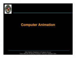
Some methods such as matrix multiplications have already been proved has more than one algorithm can be preformed. Some algorithm could be more efficient than others in theory, but not necessarily in practice. I will talk about this issue in more details later in my project. The real world Computer Linear Algebra System application such like Maple or MATLAB can do the most well known job such as Matrices problems (not only the trivial addition, multiplication but also some more complicate algorithm such as Gauss-Jordan Elimination) of computation in Linear Algebra and they even has been improved frequently and getting more powerful these days. The Computer Linear Algebra System is designed to be used as a tool to do the computing job, however, these applications even get graphic user interface these days to offer not only the good performances of the computation itself but also the more convenient way to monitor and modify the work has been done.
Figure 1.1: A typical worksheet shows in Maple 9.5 I may involved a graphic user interface into my System as well, but since most of popular Computer Linear Algebra System exists using a graphical but still command line user interface, I may just implement a simple command line based graphic user interface not only to catch up a window application standard but also make it easy to start with and familiar to modern users. Before we start everything else, we would better consider the project management details first. Such as the aim, objectives, applications, requirements specification and the project plan. A good analysis and organized project management plan, can certainly improve the efficiency and the quality of the project. So the following stage will be the project management plan of the whole process.
-7-
1.1 Aim: The aim of this project is to design and implement a simple linear algebra system which can work as a usual linear algebra system and solve some certain Linear Algebra problem. The software can be used like an alternative way of computer aided linear algebra computation for people who want to deal with some functions but don’t have to bother with other fully functional involved lager mathematic applications such as Maple. And plus this tiny small one is free. Also from this project the developer can review and learn algorithms of linear algebra computations. It is an also good programming exercise of the Java language.
1.2 Objectives: 1. To revise all the works have done in the kingdom of linear algebra, and further more to investigate any existing mathematic knowledge which is linked with a tiny computer linear algebra system. 2. To revise or study the essential programming skills which may be involved in the implementation process of the project. 3. To design and implement a small computer linear algebra application includes a reasonable user interface. 4. To identify the problems and limitations of the trivial algorisms. 5. To identify the problems with different input type may influence on the feedback and lead to the differences of the result. 6. To suggest and improve trivial algorisms in order to suit the specific problems.
1.3 Applications: Computer Linear Algebra System is not only a good practice for academic project, but also a very useful tool for lots of the applications in so many different domains. For instance the education sphere, it is easy to see Computer Linear Algebra System is an ideally tool for both the teaching and learning purpose in linear algebra kingdom. And also any industry project or laboratory researching who is dealing with a large number computation of linear algebra requires computer aided algebra system.
1.4 Project Plan 1.4.1 Project Phases The project will be split in to four distinct phases. The first phase will be a review of the background knowledge and theory. The other three, however produces a useable system by each. The different amount them is just the later stage will add on the more functions. There is an activity bar chart created by using project plan software GanttProject shows the planning of my project in appendix. Phase 1 Literature Review. -8-
Phase 2 First Prototype Includes Basic Algorithms. Phase 3 Second Prototype Includes determinants and Linearly Dependence. Phase 4 Final Prototype includes all Functions.
1.4.2 Milestones and Deliverables Deliverable 1: Report of Project Proposal Deliverable 2: Report of Literature review Milestone 1: Summary of the First Prototype Milestone 2: Summary of the Second Prototype Milestone 3: Summary of the Final Prototype Deliverable 3: Final Report
-9-
Deadline 24/10/05 Deadline 12/12/05 Deadline 19/12/05 Deadline 06/03/06 Deadline 01/05/06 Deadline 08/05/06
Chapter 2 Literature Survey
1 Introduction Mathematics is not only a discipline of its own right but also a tool used in many other fields. Linear algebra as a branch of mathematics that plays a central role in modern mathematics and also takes an important status in other major science spheres such like engineering, physics, computing and social behaviour. Computer Linear Algebra System is a computer software application aimed to helping people solve computational problems within Linear Algebra domain. It is obvious to see such a system will have a great value in both academic and commercial territory. In order to do this project successfully, we must first of all research and review the literatures and papers which related with this specific problem. Certainly, we can make the dream to be true, because a huge amount of work has been done by numbers of admirable scientists and boffins in both mathematic and computer science domain. And also some computer aimed mathematical tools has been successfully released by a number of computer experts lead to a significant improvement in all relative science domain and even our social life. Thanks all of these predecessors leave us a considerable large scope of knowledge to be learning and dealing with. However, rests with our problem I am going to talk bout mainly 3 spheres of them: 1. The Linear Algebra algorithms are clearly the theoretical background of the whole System. Some algebra problems such as addition of Matrices may be considered before the others as a basis of more advanced algorithms. 2. The real world mathematic products which show good examples for our argument and also give us a direction to follow up and even could be a starting point to go further. 3. Last but not least, try to use some advanced algorithms to solve the linear algebra problems.
2 Linear Algebra Linear algebra is a mathematics branch concerned with the study of vectors, vector spaces, matrices, linear transformations, and systems of linear equations. Let’s first of all consider the matrices and the vectors. Since prehistoric times, Latin squares and Magic squares have been studied. The origins of mathematical matrices lie with the study of systems of simultaneous linear equations. An important Chinese text from between 300 BC and AD 200, Nine Chapters of the Mathematical Art, gives the first known example of the use of matrix
- 10 -
methods to solve simultaneous equations. The theory of determinants developed in 1693 by one of the founders of calculus Leibniz. Cramer developed the theory further, presenting Cramer's rule in 1750. In the 1800s, Carl Friedrich Gauss and Wilhelm Jordan developed Gauss-Jordan elimination. (Laura Ackerman Smoller, 2005) Before we deal with the computational problems of matrices, we should first of all declare what is a matrix. Also describe some definition for the further explanation of the algorithms in later stage. A matrix is a rectangular array of numbers. The numbers in the array are called the elements of the matrix. The horizontal lines in a matrix are called rows of a matrix and the vertical lines are called columns. A matrix with m rows and n columns is called m×n matrix. The element of a matrix A that lies in the ith row and the jth column is called the i,j element or (i,j) th element of A. This is written as A[i,j] or ai,j in my follow description. (Gareth Williams, 2001) Here is an example shows a 4×3 matrix called A.
A is a 4×3 matrix, the element A[3,1] or a3,1 is 4 If the number of rows m is equal to the number of columns n, A is said to be a square matrix. A submatrix of a given matrix is an array obtained by deleting certain rows and columns. For example there is a matrix A:
If we build a submatrix of A by deleting the row 3 and column 2 we got the following submatrix of A
- 11 -
An identity matrix is a square matrix with 1s in the diagonal locations (1,1) ,(2,2) ,(3,3), and so on and zeros elsewhere. We write In for the n×n identity matrix. For example the following matrices are identity matrices.’
(Wikipedia, 2005)
2.1 Addition of Matrices Let A and B be matrices of the same size. Their sum A + B is the matrix obtained by adding together the corresponding elements of A and B. The matrix A + B will be of the same size as A and B. (Gareth Williams, 2001) For example:
(Wikipedia, 2005)
2.2 Scalar Multiplication of Matrices Let A be a matrix and c be a scalar. The scalar multiple of A by c, denoted cA, is the matrix obtained by multiplying every element of A by c. The matrix cA will be the same size as A. (Gareth Williams, 2001) For example:
Let A, B and C be matrices and a, b, and c be scalars. Assume that the sizes of the matrices are such that the operations can performed. Matrix Addition and Scalar Multiplication have following properties 1. 2. 3. 4.
A+B=B+A A + (B + C) = (A + B) + C A+O=O+A=A c(A + B) = cA + cB
where O is the appropriate zero matrix
- 12 -
5. (a + b)C = aC + bC 6. (ab)C = a(bC)
2.3 Negation and Subtraction We now define subtraction of matrices in such a way that makes it compatible with addition, scalar multiplication, and negation. Let A - B = A + (-1) B (Gareth Williams, 2001)
2.4 Multiplication of Matrices Let the number of columns in a matrix A be the same as the number of rows in a matrix B. the product AB then exists. The element in row i and column j of AB is obtained by multiplying the corresponding elements of row i of A and column j of B and adding the products. (Gareth Williams, 2001) Let A have n columns and B have n rows. The ith row of A is [ai1, ai2…ain] and the jth column of B is [b1j, b2j…bnj]. Thus if C = AB, then cij = ai1b1j + ai2b2j + … + ainbnj. For example
Let A, B and C be matrices and a, b, and c be scalars. Assume that the sizes of the matrices are such that the operations can performed. Matrix Multiplication has following properties 1. A(BC) = (AB)C 2. A(B + C) = AB + AC 3. (A + B)C = AC + BC 4. AIn = InA = A 5. c(AB) = (cA)B = A(cB) Note: AB ≠ BA in general
where In is the appropriate identity matrix
Some important Properties of Matrix Multiplications may lead to different efficiency during the multiplying chain matrices. We are going talk about it separately in later stage.
2.5 Transpose The transpose of a matrix A, denoted At, is the matrix whose columns are the rows of the given matrix A. (Gareth Williams, 2001) For example - 13 -
Properties of Transpose Let A and B be matrices and c be a scalar. Assume that the sizes of the matrices are such that the operations can performed. 1. 2. 3. 4.
(A + B)t = At + Bt (cA)t = cAt (AB)t = BtAt (At)t = A
A symmetric matrix is a matrix that is equal to its transpose.
2.6 Trace Let A be a square matrix. The trace of A, denoted tr(A) is the sum of the diagonal elements of A. thus if A is an n×n matrix, tr(A) = a11 + a22 + … + ann (Gareth Williams, 2001) Properties of Trace Let A and B be matrices and c be a scalar. Assume that the sizes of the matrices are such that the operations can performed. 1. 2. 3. 4.
tr(A + B) = tr(A) + tr(B) tr(AB) = tr(BA) tr(cA) = ctr(A) tr(At) = tr(A)
2.7 Matrices with Complex Elements The elements of a matrix may be complex numbers. A complex number is of the form z = a + bi Where a and b are real numbers and i = √-1. a is called the real part and b the imaginary part of z. (Gareth Williams, 2001) Let z1 = a + bi, z2 = c + di be complex numbers. The rules of arithmetic for complex numbers are as follows.
- 14 -
Equality: Addition: Subtraction: Multiplication:
z1 = z2 if a = c and b = d z1 + z2 = (a + c) + (b + d)i z1 – z2 = (a – c) + (b – d)i z1z2 = (a + bi)(c + di) = a(c + di) + bi(c + di) = ac + adi + bci + bdi2 = ac + bdi2 + (ad + cb)i = (ac – bd) + (ad + cb)i
The conjugate of a complex number z = a + bi is defined and written z’ = a – bi. The conjugate of a matrix A is denoted and A is obtained by taking the conjugate of each element of the matrix. The conjugate transpose of A is written and defined by A* = A’ t Properties of Conjugate Transpose Let A and B be matrices with complex elements and let z be a complex number. 1. (A + B)* = A* + B* 2. (zA)* = z’A* 3. (AB)* = B*A* 4. (A*)* = A
2.8 Gauss-Jordan Elimination & System of Linear Equations Gauss-Jordan Elimination are widely used in linear algebra for determine the solutions of a system of linear equations, for determining the rank of a matrix, and for calculating the inverse of an invertible square matrix. Gauss-Jordan Elimination can be used to determine the solutions of a system of linear equations. When we apply it to a matrix it produces a reduced echelon form. For example we have linear equations: 2x + y − z = 8 − 3x − y + 2z = − 11 − 2x + y + 2z = − 3 This is called a system of linear equations for the unknowns x, y, and z. If we can transform it into another equivalent one so that we can easily see the solution, should be a good way to find the solution. The operations to transform a system of equations to another are as follows: 1. Interchange two equations 2. Multiply or divide both side of an equation by a non-zero constant 3. Add or subtract a multiple of one equation to another one
- 15 -
Ideally, if linear equations system after transformation contains x only in first equation, y only in second equation, z only in third equation, then we can easily read the solutions. After we do so we finally get X=2 Y=3 Z=1 Instead of deal with the system of linear equations, we can do it by only consider the augmented matrix. The augmented matrix of a linear equations system is just combine the coefficients, together with the constant terms, form a matrix. For example the augmented matrix of the linear equations system above is
Similar here we can 1. Interchange two rows. 2. Multiply or divide the element of a row by a nonzero constant. 3. Add multiple of elements of one row to the corresponding elements of another row. Finally we have
This matrix shows the same solution by the last column and also it is in reduced echelon form. A matrix is in reduced echelon form also called reduced row-echelon form if 1. Any rows consisting entirely of zeros are grouped at the bottom of the matrix. 2. The first nonzero element of each other row is 1. This element is called a leading 1. 3. The leading 1 of each row after the first is positioned to the right of the leading 1 of the previous row. 4. All other elements in a column that contains a leading 1 are zero. (Gareth Williams, 2001) We now summarized the method the method we use above to find out the reduced echelon form, it’s called Gauss-Jordan Elimination.
- 16 -
Gauss-Jordan Elimination 1. Write down the augmented matrix of the system of linear equations. 2. Derive the reduced echelon form of the augmented matrix using elementary row operations. This is done by creating leading 1s, then zeros above and below each leading 1, column by column starting with the first column. 3. Write down the system of equations corresponding to the reduced echelon form. This system gives the solution. (Gareth Williams, 2001) Note there are three possibilities when solving system of linear equations. They are unique solution just like we described above, and also no solution and many solutions. No solution means there is no value for unknowns satisfies all equations simultaneously. For example
This matrix represents a system of linear equations has no solutions. Because the third row gives the equation 0 = 1, which can never be satisfied. Many solutions means there are many possible values for owns satisfies all equations simultaneously. For example
This matrix represents equation x + (2/3)y = 11 and z = 7, we can have many in fact infinite numbers of solutions for x and y satisfy the equations.
2.9 Inverse of matrix Let A be an n×n matrix. If a matrix B can be found such AB = BA = In, then A is said to be invertible and B is called the inverse of A. If such a matrix B does not exist, then A has no inverse. (Gareth Williams, 2001) The inverse of an invertible matrix is unique. We can also use Gauss-Jordan Elimination to finding the inverse of a matrix as we mentioned before. 1. Let A be an n×n matrix In to A to form the matrix [A:In]. 2. Compute the reduced echelon form of [A:In]. If the reduced echelon form is of the type [In:B], then B is the inverse of A. If the reduced echelon form is not of the type [In:B], in that the first n×n submatrix is not In, then A has no inverse. - 17 -
An n×n matrix A is invertible if and only if its reduced echelon form is In. (Gareth Williams, 2001)
2.10 Determinant The determinant of a 2×2 matrix A is denoted det(A) or |A| and is given by
Observe that the determinant of a 2×2 matrix is given by the difference of the products of the two diagonals of the matrix. Let A be a square matrix. The minor of the element aij is denoted Mij and is the determinant of the matrix that remains after deleting row i and column j of A. The cofactor of aij is denoted Cij and is given by Cij = (-1)i+jMij The determinant of a squire matrix is the sum of the products of the elements of any row or column and their cofactors. ith row expansion: jth column expansion:
|A| = ai1C i1 + ai2C i2 + … + ainCin |A| = a1jC1j + a2jC2j + … + a3jC3j
2.11 Rank The dimension of the row space and the column space of a matrix A is called the rank of A. the rank of A is denoted rank(A). (Gareth Williams, 2001) The easiest way to compute the rank of a matrix A is given by the Gauss elimination method. The row-echelon form of A produced by the Gauss algorithm has the same rank as A, and its rank can be read off as the number of non-zero rows. Consider for example the 4 by 4 matrix:
- 18 -
We see that the second column is twice the first column, and that the fourth column equals the sum of the first and the third. The first and the third columns are linearly independent, so the rank of A is two. This can be confirmed with the Gauss algorithm. It produces the following row echelon form of A:
which has two non-zero rows. (Wikipedia, 2005)
3 Computer Algebra Systems In order to understand which kind of software we are dealing with. We’d better look at the solutions of these problems around first. Since mathematics are the foundation of almost all science subjects, not only more and more computer algebra system are released these days to suit this trend, but also getting more powerful. Computer algebra systems firstly appeared in 1970s, and were aimed for helping Artificial Intelligence research, although these days become a powerful tool in much more fields. REDUCE1, Derive2, and Macsyma3 were the first popular systems, and there is a free version of Macsyma called Maxima4 still active. Maple and Mathematica are the market leader today and both of them are commonly used by research mathematicians, scientists, and engineers. We are going to talk about those two applications in more details later on as the case study representatives. (Dan Ginsburg 2001), (Wikipedia, 2005), (Freek Wiedijk, 2005) Worth to point out that some computer algebra systems focus on a specific area of application, these are typically developed in academia and free. My project is just one of those which focus on the linear algebra problems. (Wikipedia, 2005)
3.1 Maple Maple is a general purpose commercial computer algebra system. It was first developed in 1980 – 1981 by the Symbolic Computation Group at the University of Waterloo in Waterloo, Ontario, Canada. Since 1988, it has been developed and sold commercially by Maplesoft, a division of Waterloo Maple Inc. A Canadian company also located in Waterloo, Ontario. The latest version so far is Maple 10. (The Symbolic Computation Group, 1993) ‘Maple is the ultimate productivity tool for solving mathematical problems and creating interactive technical applications. Intuitive and easy to use, it delivers the
- 19 -
most advanced, complete, reliable mathematical capabilities that can only come from a market-leading tool that has been developed and tested over 25 years. Maple allows you to create rich, executable technical documents that provide both the answer and the thinking behind the analysis. Maple documents seamlessly combine numeric and symbolic calculations, explorations, mathematical notation, documentation, buttons and sliders, graphics, and animations that can be shared and reused by your colleagues.’ (Maplesoft, 2005) Let’s now see the features of Maple Maple includes over 3,500 computational functions to deliver the richest set of computation tools for any area in mathematics, science, or engineering. Although the major topics of Maple are Algebra, Calculus, Differential Equations, Linear Algebra, Solvers, Statistics, Vector Calculus, it can also deal with a huge amount of other problems such as Abstract Algebra, Combinatorial Functions, Curve, Fitting, Differential Algebra, Financial Mathematics, Gaussian Integers, Graph Theory, Groebner Bases and Polynomial Ideals, Group Theory, Logic, Number Theory and so on. It’s easy to see Maple is not only a powerful in linear algebra kingdom which is what we are interested in, but also a really good computer algebra systems in a large separate fields. It can be use to solve all the linear algebra problems as for as I know. But Can I do it even better? To do the linear algebra computation with maple is convenient. We just need to input the command after a maple input symbol ‘[>’, then we will get the response relative to the order in next a few lines. Note all the maple input line must end with a semicolon ‘;’ otherwise it will not be accept. In the new version of Maple, release 10. There are even more convenient way to deal with the problems we can simply choose the functions we want to use in a Matrix Palette contains. And also it seems to be improved the documentation feature. People do not have to input maple commend began with symbol ‘[>’, but tell Maple this is maple input line or a plain text line instead. (Maplesoft, 2005)
3.2 Mathematica Mathematica is another widely used computer algebra system originally developed by Stephen Wolfram and sold by his company Wolfram Research. The first version was developed by Stephen Wolfram and released in 1988. The latest version is Mathematica 5.2. (Wikipedia, 2005)
- 20 -
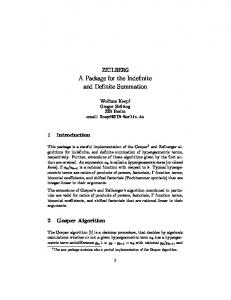
‘From simple calculator operations to large-scale programming and interactivedocument preparation, Mathematica is the tool of choice at the frontiers of scientific research, in engineering analysis and modelling, in technical education from high school to graduate school, and wherever quantitative methods are used.’ – The way Wolfram Research, Inc. describes their produce.
Figure 2.1: Pie chart of Mathematica user’s domain (Wolfram Research, 2005) Again Mathematica also provide the most commonly know Matrix Operations such as compute Inverse, Transpose, determinants of a given matrix. For example the following Mathematica input will find the determinant of the 6×6 matrix whose i, jth element contains ij with all zero elements replaced as 1. In[1]:= Det@ReplaceAll[Table[i j, {i,0,5}, {j,0,5}],{0->1}] Out[1]= 0
3.3 MATLAB Again another powerful tool is MATLAB. It’s a numerical computing environment and also a programming language. MATLAB allows easy matrix manipulation, plotting of functions and data, implementation of algorithms, creation of user interfaces, and interfacing with programs in other languages. It is also a full computer algebra system by involve a Maple symbolic engine. It is used by over one million people in industry and academia. It can be run on the different modern platforms such as Windows, Mac OS, UNIX and Linux. However it is just as expensive as other software applications charge approximately US$2000 for commercial use and US$100 for an academic license with a limited set of Toolboxes. (Wikipedia, 2005) MATLAB short for ‘Matrix Laboratory’, it was invented in the late 1970s by Cleve Moler. Later pass to the leader of the computer science department at the University of New Mexico. It was originally designed it to let students access to LINPACK and EISPACK without having to learn FORTRAN. The MathWorks start to maintain the - 21 -
software in 1984. MATLAB was first adopted by control design engineers, but quickly spread to many other domains. It is now also used as a tool to teaching of linear algebra and numerical analysis in education. (Wikipedia, 2005) On their own web page they describe their product like this ‘MATLAB is a high-level technical computing language and interactive environment for algorithm development, data visualization, data analysis, and numeric computation. Using MATLAB, you can solve technical computing problems faster than with traditional programming languages, such as C, C++, and FORTRAN. You can use MATLAB in a wide range of applications, including signal and image processing, communications, control design, test and measurement, financial modelling and analysis, and computational biology. Add-on toolboxes (collections of special-purpose MATLAB functions, available separately) extend the MATLAB environment to solve particular classes of problems in these application areas. MATLAB provides a number of features for documenting and sharing your work. You can integrate your MATLAB code with other languages and applications, and distribute your MATLAB algorithms and applications.’ (The MathWorks, 2005) MATLAB offer a good Function Reference which we can access and learn the use of the software and even some algorithms undertaking easily. For example this is the MATLAB Function Reference for calculate determinant of a matrix.
det Matrix determinant
Syntax • •
d = det(X)
Description d = det(X) returns the determinant of the square matrix X. If X contains only integer entries, the result d is also an integer.
Remarks Using det(X) == 0 as a test for matrix singularity is appropriate only for matrices of modest order with small integer entries. Testing singularity using abs(det(X)) =p2.size Add p1[i] to res. Else Add p1[i]+p2[i] to res. End for Return res;
polyMulti This method multiplies two polynomial’s coefficients list together. It is very important function for the characteristic polynomial calculation in this system. Input: Integer list: p1, p2 Output: Integer list: res Pre-condition: None Post-condition: Return a list which is the result of multiplying two polynomial’s coefficients list together.
Algorithm: Let p1 be the list contains coefficients of a polynomial. Let p2 be the list contains coefficients of another polynomial. Create an empty integer list res. For i = 0 to p1.size-1 For j = 0 to p2.size-1 If current res.sizej,U[i][j] = 0; When i=j,U[i][j] = 1; When i>’ just like MATLAB. After compare among the exciting user interfaces, the developer designed to use a simply user interface just like MATLAB. All the available commands are listed below: add: minus:
Adding two matrices together. Subtract a matrix from another.
- 75 -
multi1: multi2: multi3: load: save: clc: who: det: trace: rank: rand: solve1: solve2: solve3: solve4: solve5: adj: chc: inv1: inv2: clear: row: col: set: ref: equals: syc:
Calculating the product of two matrices use definition matrix multiplication algorithm. Calculating the product of two matrices use Strassen algorithm. Calculating the product of two matrices use Winograds algorithm. Load the content of filename into a matrix named matrixname. When matrixname omitted, it will be assumed to be the filename. Store the value of matrixname into a file named filename. When filename omitted, it will be assumed to be "matrixname.out". Clear the command window. Display the variables which have been defined. The determinant of square matrix A. The trace of the matrix. Rank of a matrix. Generate a random matrix m by n, each element is a uniform distributed random integer ranged 0 to r. Use inverse algorithm to solve a linear equations system. Use Gauss-Jordan elimination algorithm. Use Gausselimination algorithm. Use LU decomposition. Use Gauss-Jordan elimination, but can deal with the case in which there is no solution or many solutions. Calculate the adjoint of matrix. Calculate the characteristic polynomial of matrix. Calculate the inverse of matrix using Gauss-Jordan elimination algorithm. Calculate the inverse of matrix using adjoint of matrix. Delete all variable in the matrix system or if followed by a parameter delete the selected variable. Get row number of matrix. Get column number of matrix. Re-set a value to a element of matrix. Get the reduced echelon form of matrix Check to see if two matrices are equal. Check to see if matrix is symmetric.
A more convenient way to get use to the system is using the build in help system. Whenever a user type in command ‘help’, there will be a whole list of the commands available appear on the screen. Further more by using ‘help ’ syntax with a specific command as the parameter, the user will get the information and introduction of the selected command.
- 76 -
Figure 5.2: Build in help system
The command widow can be dragged to anywhere on the screen and the size of the window can be easily modified just like any other windows. Although this simple user interface still has some weak point, it is easy to use, easy to learn and focus on the target tasks of the system. It is simply but not bad.
- 77 -
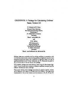
Figure 5.3: Create two matrices and add them together
4.3.2 Implementation of the user interface There are three classes in this package MatrixSystem, SymbolEntry and Util. this package not only just an interface implementation of the system, but also the application of the kernel. MatrixSystem have the most methods for running the user interface. SymbolEntry class creating the SymbolEntry objects for keeping the variables in the system.
4.3.2.1 Util class util class contains explanations strings for the help command, those strings shows on the screens when user type in ‘help’ commend. This class has only one impartment method parse
parse This method parses and classifies the numbers in command line strings into three different Number types of the system: Int, Doub and Fraction. The trick is check the string, if it contains symbol ‘/’ than it is a Fraction, else if it contains symbol ‘.’ It should be a Doub, else it is an Int.
- 78 -
Input: String Output: Number Pre-condition: None. Post-condition: It returns a Number object by parsing the number information in command.
4.3.2.2 SymbolEntry class This class creating the important SymbolEntry objects, each SymbolEntry object contains either a Number or a Matrix objects with a name. Every operand keep in the system is a SymbolEntry objects. Creating such objects is the main task of this class. It is obvious this class should contain two constructors: ‘SymbolEntry(Matrix symbol, String name)’ and ‘SymbolEntry(Number n, String name)’ For two different type of operands Matrix and Number.
4.3.2.3 MatrixSystem class This is the main class of the user interface system. It contains almost all implementations of the user interface. Since the user interface of the system is very simple only contains a JTextArea called command window and a JScrollPane for scroll the screen up and down when command window has been crammed. All the operations are done in the command window by type in the commands. The biggest issue is how to pass a command into the kernel of the system.
parseCommand This is the method that parses a command typed in by a user and calls the related algorithm method in the core package. Input: String Output: None Pre-condition: None Post-condition: It prints out the operation result on the screen if the command is in the correct format and records some of them for future use. The method parses and identifies which command has been typed in, than check the syntax of the command and the syntax of the validity of the parameters. When all the conditions agree with the specific command syntax requirements, it will call the algorisms regarding to the command. Therefore, the results of the operation will be print on the screen and may be recorded for the future use. Since it works in a trivial and mechanical way, I will only give an example of the ‘add’ command. When user type in a command line contains string ‘add’, it will switch to the processing of ‘add’ condition. Firstly, check if the input is in accord with the syntax of ‘add’ command. Secondly, check if the number of arguments is two which meets - 79 -
the syntax requirements. Thirdly, check if the arguments exist in the system. Since two different types Matrix and Number object can not add together, than it checks if two arguments have the same type. If everything up to here meet the perfect condition, it will invoke one of the two different add method for Matrix or Number depending on the type of the arguments. Finally, it prints out the result on the screen and record the answer in to a SymbolEntry object called ‘ans’.
findSymbol The method searches symbolList and finds out the SymbolEntry object wanted in the symbolList, than returns it. Returns null if it is not there. Input: String Output: SymbolEntry Pre-condition: None Post-condition: It finds and returns a SymbolEntry object, return null if not there.
4.4 Evaluation & Testing In order to go further without many errors, the project has been tested carefully during the implementation process. However, it is almost imposable to record and document all the testing has been done. Also, to perform a fully testing meet the industry software engineering requirement is quite time consuming. So finally the developer decide to provide a reasonable testing plan which contain all the main algorithms implemented in the kernel of the system, and also cover all the different data types involved in to the system. In order to make sure the testing has an acceptable efficiency, some of the testing strategies will be involved. The counterexamples against the pre-conditions of the methods will be tested. The type compatibility of the system will be tested. For example, two matrices can only add together when they have exactly the same size, so the different size matrices will be try to added during the process, see the if the system will catch the problem and trade it correctly. There will be no extremely large matrices involved into the testing plan, since the result is difficult to handle and the algorithms errors can also be targeted in small matrices. Unfortunately, the user interface will not be formal test and reported, because of the time issue. It has been tested informally by the developer and the main problems have been fixed. Since the user interface involved in the system is remains simple, it has no interview or questionnaire evaluation by inviting the different group of users. The full testing plan of the system will be found in the appendix. There will be five sections for each single test, the test number, testing method, input of the specific test, Expected Output and the actual output of the test.
- 80 -
Chapter 5 Critical Evaluation & Conclusion The final important part of the project is the Critical Evaluation. This evaluation looks into the different part of the process, identify those goals that were achieved and some could be improved. It analyses the decisions made, the design and the advantage and disadvantage of the system. The system has been designed to be implemented as two components: the kernel, which is the engine of the whole system, contains all the algorithms of the computations and the user interface. So they can be redesigned and implemented separately, which improved the expansibility of the system. All of them are implemented by using the object oriented programming language Java. It has some obvious advantages such as the portability. The system has never been tested under other platforms rather than Microsoft Windows, but as java is designed for ‘implemented once and run anywhere’ it should be easily transplant to other operating systems or even running on the internet web page. The further work for the portability issue will leave to the other who wants to continue. However, Java also brings some disadvantages in to the system. The efficiency of the language is an example. Some advanced method for high computation efficiency purpose even slower than the original method, such as the fast multiplication method use Strassens algorithm. It could be the problem caused by the Java language. Strassens algorithm need to recursively call the method itself until the matrix cannot be divided further as the algorithm require. It seems to be more efficient way of calculating by the theory described in the Literature Survey chapter. But since the method call in Java consumes much more system resources than those saved by advanced algorithm, it actually even slows the progress down in the practice. That is also why sometimes I try to re-coding the whole algorithm in some method again rather than just call other methods existing performing exactly the same procedure. There are two ways to solve this problem I can suggest as this stage. They are improving the Java running efficiency by the engineers of Sun Microsystems or implementing the system by using another programming langue that have a higher operational efficiency. The system is eventually compatible with different data types such as integer, double and fraction. It increases the accuracy of the system significantly. Every integer or fraction elements in matrix will be calculated accurately instant of approximate real number answer. The initial prototype can only deal with the matrix with double type elements. At this stage, all the methods were implemented for the real number input only. And the data structure of the matrix is quite simple just a 2D double array and a name. After the most of operational methods have been successfully implemented and tested, I decide to improve the system compatibility for the accuracy issue. Firstly, I tried to integrate the integer type in to the system in order to get the accuracy answer for the integer matrices calculation.
- 81 -
However there are a few problems appearing immediately. One is the data stricture, if it remains unchanged but add a new constrictor for integer element matrix, than all the method have to be implemented twice for the compatibility problem. It is also deal with the matrix with integer and real number elements mixed as a double matrix. Further more integers are easily transformed to non-integer numbers during the computation progress. For example, when 2 divided by 3 the answer will be a problem. So the system had to be redesigned again. The final prototype is this one user can deal with. The design has been changed to use a slightly more complex data abstract. Every element of a matrix is an object called Number, and each Number could be one of the three different number type integer, double and fraction. A complex number is just a combination of real part and imaginary part as described in Literature Survey section, and all real numbers is just a complex number with the imaginary part equals to zero. So that any real numbers compute with a complex number could get a complex number answer. However two complex numbers with opposite imaginary part numbers add together will get a real number. I will leave this part to the further improvement after this project, since I have no time to deal with it. The design has some obvious advantages. Because the fundamental computations between two elements are independent from the matrix, all the arithmetic algorithms between to matrices just need to be implemented once for the parent type Number. On the other hand, since fraction type has been involved, the arithmetic between integers or fractions can now have the exact answer. Further more Matrices themselves are free of the bundle with the element type, which means different type of numbers can now be allocated into one single matrix. It gets the greatly Profit from this data abstract. The system can now be improved further easily. For instance, expands the compatibility to involve other number types such as complex without a great difficulty. However, the design brings some pains. It may lead to the low operational efficiency even lower. Not only because there is a type checking during parsing stage but also a return type selections during the arithmetic operation process. The simple types of Java like integer has been re-packaged into a new Int object may also slow the whole process down. The design is not perfect. When the computations involve double numbers, the accuracy remains low. Users can easily see that in the testing plan & results in appendix, inaccuracy appeared at a high possibility when dealing with the real numbers. The result numbers like 0.19999999999999996 which should be 0.2 in accurate computation still exists. It is meanly because the approximate calculating results run through the whole operational process make the answer become imprecise, especially in the complicated algorithms such as calculating detrminants. It is sometimes called round-off errors. Also it might be because of the way of number representing in the computer. Unlike other applications, this system keeps all the matrix functional algorithms in one class: matrix. I decided not to separate the matrix class into pieces in which each
- 82 -
class contains different group of functional method, but package everything together it is because all the operation in matrix performing on the matrix object. I manage the system in this way reflecting the object oriented programming thinking, and take advantage of the object oriented programming benefit. Another characteristic feature of the system is it can construct and store the unlimited large matrices. Although the 2D array itself is not increasable, but because the number of rows and columns of matrix get while parsing, the size of the 2D array can be set just as large as the matrix. When reading from a file, I use an ArrayList has ArrayList elements, use this way to create a dynamically memory allocated 2D array. Therefore the system can add the next element to the inner ArrayList one after another, than add the rows to the outer ArrayList one after another finally create a new matrix object. So the maximum matrix size will be imposed by the machine running the system rather than the system itself. Also the system can store unlimited many matrix object in the memory list because it is an ArrayList again. The more algorithms can be added to the system, for example use iterative method to solve the system of linear equations, such as the Jacobi method. It is not difficult to add such kind of new algorithms in to the system since my system have a good expansibility profit from the design of the system structure. And also it is possible to work out the Eigenvalues and Eigenvectors of a matrix since we have already got the characteristic polynomial of matrix. The problem is characteristic equations could be a high dimension equation. We all know that there is not a specific formula for solving the equations with dimensions over five. Therefore we can only have the approximate solutions. Also there are other algorithms have been reviewed in the Literature Survey stage but never been implemented such as Matrices Chain Multiplication. Some algorithms the developer has now got the ideas after the implementation of the system such as iterative methods for solving systems of linear equations, typically Jacobi Method and Gauss-Seidel Method. They can also be integrated into this system. So this part I left as a further work for others continue again, since I have not enough time. The user interface of the system has been developed as well. However I just decided to keep it simple since the good looking graphical user interface not help much for user who wants to deal with the mathematical problems but slow down the system on the other hand. The user interface is just a command window, users need to type in the command by them, if anybody thinks there could be an improvement at this user interface than I will just give some suggestions now. The system can only read the command at the left side of the prompt, whenever a user press ‘Enter’ button. If the prompt is not allocated at the end of the entire command line, the system will just place prompt to a new line. It could be improved by further work. Since the symbol ‘>’ have been used as a starting symbol, the system cannot delete any ‘>’ typed in by user either, that means every time a user type in ‘>’ must re type the whole command rather than modify it by pressing on backspace. The system allow user to choose a specific algorithm among several different algorithm for the same operations, this design allow user to compare the algorithms
- 83 -
efficiency of the system. However, the system did not provide the function which automatically chooses the best method for the user. There is a help system integrated in the system, and it makes anyone can easily get use to the system in a very short time. There could be a dramatically improving of the system usability, if it allowed user to performing and operations by just pass in the real parameters instead of the matrix have already been added in to the object list. For example, add(3, 5) or even 3 + 5. But, it is not as simple as it looks like. It could raise the complexity of the command parser implementation rapidly. Since if we want the system to understand det(inv(((5+4)/4+6*(9-3))*[1,2;3,4])), than we might need to implement a compiler for the system first of all. I have no time to deal with such kind of problem, so again leave it to others. The system can read and write the matrices form and to a file. This feature improved the usability of the system, since user can input large matrices in a convenient way by pre-store it in to a file. And also user can save a large computation result to a file for storing or re-using purpose. However, the system now can only read the file which contains only one matrix in such a simple structure: one line of the text file contains only one row of matrix in correct order and elements in a row are separated by the spaces, that means the matrix is represented in the same way as it should be represented on a piece of paper but without brackets. So it is not so convenient for user who wants to input a large amount of matrices or save more than once. If the system can accept a more completed and structured file format and a more reasonable output would be great for the further improving of the usability. I have to say sorry this function will leave to the other people again. The system can now automatically remember the last computation result and keep it in system called ‘ans’. This feature improves the usability obviously, since people always want to re-use the result of the last computation for the next calculating. But it is not good enough, of the system can remember a number of results may make this feature more valuable. Now, the project is done. Although the further work still needs, almost all the requirements have been met. So I can say this project has been done successfully to some degree.
- 84 -
Reference & Bibliography Dan Ginsburg (2001), Brian Groose, Josh Taylor, Prof. Bogdan Vernescu, Advisor, ‘The History of the Calculus and the Development of Computer Algebra Systems’, Department of Mathematical Sciences - Worcester Polytechnic Institute, Worcester, available from Internet [http://www.math.wpi.edu/IQP/BVCalcHist/calctoc.html] Freek Wiedijk (2005), Radboud University Nijmegen, Nijmegen The Netherlands, available from Internet [http://www.cs.ru.nl/~freek/digimath/] Gareth Williams (2001), Linear Algebra with Applications fourth edition, Jones and Bartlett Publishers, Sudbury, Massachusetts Laura Ackerman Smoller (2005), Department of History, University of Arkansas at Little Rock, available from Internet [http://www.ualr.edu/~lasmoller/matrices.html] Maplesoft (2005), a division of Waterloo Maple Inc, available from Internet [http://www.maplesoft.com/products/maple/index.aspx] STAT-NCTU (2006), ‘LU decomposition’, National Chiao-Tung University Institutes of Statistics Bioinformatics and Medical Images Stat. Group, available from Internet http://www.stat.nctu.edu.tw/MISG/SUmmer_Course/C_language/Ch06/LUdecomposi tion.htm The MathWorks (2005), Inc, Natick, Massachusetts, available from Internet [http://www.mathworks.com/products/matlab/description1.html] The Symbolic Computation Group (1993), ‘History of Maple’, School of Computer Science, Faculty of Mathematics, University of Waterloo, Waterloo, Ontario, Canada, available from Internet [http://www.scg.uwaterloo.ca/SCG/history.html] Thomas H. Cormen (2001), Charles E. Leiserson, Ronald L. Rivest, Introduction to Algorithms, The MIT Press, McGraw-Hill Book Company Wikipedia (2005), Wikimedia Foundation, Inc, available from Internet [http://en.wikipedia.org/wiki/Main_Page] Wolfram Research (2005), Inc, Oxfordshire, OX29 8RY, UNITED KINGDOM, available from Internet [http://www.wolfram.com/products/mathematica/index.html]
- 85 -
- 86 -