Hindawi Publishing Corporation Mathematical Problems in Engineering Volume 2016, Article ID 9329812, 14 pages http://dx.doi.org/10.1155/2016/9329812
Research Article Binary Classification of Multigranulation Searching Algorithm Based on Probabilistic Decision Qinghua Zhang1,2 and Tao Zhang1 1
The Chongqing Key Laboratory of Computational Intelligence, Chongqing University of Posts and Telecommunications, Chongqing 400065, China 2 School of Science, Chongqing University of Posts and Telecommunications, Chongqing 400065, China Correspondence should be addressed to Qinghua Zhang;
[email protected] Received 6 June 2016; Revised 5 September 2016; Accepted 26 September 2016 Academic Editor: Kishin Sadarangani Copyright © 2016 Q. Zhang and T. Zhang. This is an open access article distributed under the Creative Commons Attribution License, which permits unrestricted use, distribution, and reproduction in any medium, provided the original work is properly cited. Multigranulation computing, which adequately embodies the model of human intelligence in process of solving complex problems, is aimed at decomposing the complex problem into many subproblems in different granularity spaces, and then the subproblems will be solved and synthesized for obtaining the solution of original problem. In this paper, an efficient binary classification of multigranulation searching algorithm which has optimal-mathematical expectation of classification times for classifying the objects of the whole domain is established. And it can solve the binary classification problems based on both multigranulation computing mechanism and probability statistic principle, such as the blood analysis case. Given the binary classifier, the negative sample ratio, and the total number of objects in domain, this model can search the minimum mathematical expectation of classification times and the optimal classification granularity spaces for mining all the negative samples. And the experimental results demonstrate that, with the granules divided into many subgranules, the efficiency of the proposed method gradually increases and tends to be stable. In addition, the complexity for solving problem is extremely reduced.
1. Introduction With the rapid development of modern science and technology, the daily information which people are facing is dramatically increasing, and it is urgent to find a simple and effective way to process the complex information. So the rise and development of multigranulation computing [1–8] have been promoted by this demand. Information granulation had attracted researchers’ great attention since a paper that focused on discussing information on granulation published by professor Zadeh in 1997 [9]. In 1985, a paper named “Granularity” was published by Professor Hobbs in the International Joint Conference on Artificial Intelligence held in Los Angeles, United States. It focuses on the granulation of decomposition and synthesis and how to obtain and generate different granularity [10]. These studies play a leading role not only in granular computing methodology [11–17], but also in dealing with complex information [18–22]. Subsequently, the number of researches focused on granular computing
has rapidly increased. Many scholars successfully use the basic theoretical model of multigranulation computing to deal with practical problems [23–29]. Currently, multigranulation computing becomes a basic theoretical model to solve the complex problems and discover knowledge from mass information [30, 31]. Multigranulation computing method is mainly aimed to establish a multilevels or multidimensional computing model, and then we need to find the solving way and synthesis strategies in different granularity spaces for solving complex problem. Complex information will be subdivided into lots of simple information in the different granularity spaces [32–35]; then, effective solutions will be obtained by data mining and knowledge discovery techniques to deal with simple information. So it can solve the complex problems in different granularity or dimensions. Aiming at large-scale binary classification problem, it is an important issue to determine the class of all objects in domain by using as little times as possible. And this issue attracts a large number of
2 researchers’ attention [36–39]. Supposing we have a binary classification algorithm and 𝑁 is the number of all objects in domain and 𝑝 is the probability of negative samples in domain. Then we need to give the class of all objects in domain. The traditional method will search each object one by one by the binary classification algorithm and it is simple but has many heavy workloads when facing a large number of objects set. Therefore, some researchers have proposed group classification that each object is composed of a lot of samples, and this method improves the searching efficiency [40–42]. For example, how can we effectively complete the binary classification tasks with minimum classification times when facing the massive blood analysis? The traditional method is to test per person once. However, it is a heavy workload when facing many thousands of objects. But, to a certain extent, the single-level granulation method (namely, single-level group testing method) can reduce the workload. In 1986, Professor Mingmin and Junli proposed that using the single-level group testing method can reduce the workloads of massive blood analysis when the prevalence rate 𝑝 of a sickness is less than about 0.3 [43]. In this method, all objects will be subdivided into many small subgroups, and then every subgroup will be tested. If the testing result of a subgroup is sickness, we will diagnose the result of each object by testing all the objects in this subgroup one by one. Else if its result is health, we can diagnose that all objects in this subgroup are heathy. But for millions and even billions of objects, can this kind of single-level granulation method still effectively solve the complex problem? At present, there are lots of methods about the single-level granulation searching model [44–54], but the studies on the multilevels granulation searching model are few [55–59]. A binary classification of multilevels granulation searching algorithm, namely, establishing an efficient multigranulation binary classification searching model based on hierarchical quotient space structure, is proposed in this paper. This algorithm combines the falsity and truth preserving principles in quotient space theory and mathematical expectations theory. Obviously, on the assuming that 𝑝 is the probability of negative samples in domain, the smaller 𝑝, the higher efficiency of this algorithm. A large number of experimental results indicate that the proposed algorithm has high efficiency and universality. The rest of this paper is organized as follows. First, some preliminary concepts and conclusions are reviewed in Section 2. Then, the binary classification of multigranulation searching algorithm is proposed in Section 3. Next, the experimental analysis is discussed in Section 4. Finally, the paper is concluded in Section 5.
2. Preliminary For convenience, some preliminary concepts are reviewed or defined at first. Definition 1 (quotient space model [60]). Suppose that triplet (𝑋, 𝐹, 𝑇) describes a problem space or simply space (𝑋, 𝐹),
Mathematical Problems in Engineering where 𝑋 denotes the universe and 𝐹 is the structure of universe 𝑋. 𝑇 indicates the attributes (or features) of universe 𝑋. Suppose that 𝑋 represents the universe with the finest granularity. When we view the same universe 𝑋 from a coarser granularity, we have a coarse-granularity universe denoted by [𝑋]. Then we can have a new problem space ([𝑋], [𝐹], [𝑇]). The coarser universe [𝑋] can be defined by an equivalence relation 𝑅 on 𝑋. That is, an element in [𝑋] is equivalent to a set of elements in 𝑋, namely, an equivalence class 𝑋. So [𝑋] consists of all equivalence classes induced by 𝑅. From 𝐹 and 𝑇, we can define the corresponding [𝐹] and [𝑇]. Then we have a new space ([𝑋], [𝐹], [𝑇]) called a quotient space of original space (𝑋, 𝐹, 𝑇). Theorem 2 (falsity preserving principle [61]). If a problem [𝐴] → [𝐵] on quotient space ([𝑋], [𝐹], [𝑇]) has no solution, then problem 𝐴 → 𝐵 on its original space (𝑋, 𝐹, 𝑇) has no solution either. In other words, if 𝐴 → 𝐵 on (𝑋, 𝐹, 𝑇) has a solution, then [𝐴] → [𝐵] on ([𝑋], [𝐹], [𝑇]) has a solution as well. Theorem 3 (truth preserving principle [61]). A problem [𝐴] → [𝐵] on quotient space ([𝑋], [𝐹], [𝑇]) has a solution, if for [𝑥], ℎ−1 ([𝑥]) is a connected set on 𝑋, and problem 𝐴 → 𝐵 on (𝑋, 𝐹, 𝑇) has a solution. ℎ : 𝑋 → [𝑋] is a natural projection that is defined as follows: ℎ (𝑥) = [𝑋] , ℎ−1 (𝑢) = {𝑥 | ℎ (𝑥) ∈ 𝑢} .
(1)
Definition 4 (expectation [62]). Let 𝑋 be a discrete random variable. The expectation or mean of 𝑋 is defined as 𝜇 = 𝐸(𝑋) = ∑𝑥 𝑥𝑝(𝑋 = 𝑥), where 𝑝(𝑋 = 𝑥) is the probability of 𝑋 = 𝑥. In the case that 𝑋 takes values from an infinite number set, 𝜇 becomes an infinite series. If the series converges absolutely, we say the expectation 𝐸(𝑋) exists; otherwise, we say that the expectation of 𝑋 does not exist. Lemma 5 (see [43]). Let 𝑓𝑞 (𝑥) = 1/𝑥 + 1 − 𝑞𝑥 (𝑥 = 2, 3, 4, . . . , 𝑞 ∈ (0, 1)) be a function with integer variable. If −1 𝑓𝑞 (𝑥) < 1 always holds for all 𝑥, then 𝑞 ∈ (𝑒−𝑒 , 1). Lemma 5 is the basis of the following discussion. Lemma 6 (see [42, 63]). Let 𝑓(𝑥) = [𝑥] denote a top integral function. And let 𝑓𝑞 (𝑥) = 1/𝑥 + 1 − 𝑞𝑥 (𝑥 = 2, 3, 4, . . . , 𝑞 ∈ (0, 1)) be a function with integer variable. 𝑓𝑞 (𝑥) will reach its minimum value when 𝑥 = [1/(𝑝 + (𝑝2 /2))] or 𝑥 = [1/(𝑝 + (𝑝2 /2))] + 1, 𝑥 ∈ (1, 1 − 1/ ln 𝑞]. −1
Lemma 7. Let 𝑔(𝑥) = 𝑥𝑞𝑥 (𝑒−𝑒 < 𝑞 < 1) be a function. If 2 ≤ 𝑐 ≤ 1 − 1/ ln 𝑞 and 1 ≤ 𝑖 < 𝑐/2, then the inequality (𝑔(𝑖) + 𝑔(𝑐 − 𝑖))/2 ≤ (𝑔((𝑐 − 1)/2) + 𝑔((𝑐 + 1)/2))/2 < 𝑔(𝑐/2) holds.
Mathematical Problems in Engineering
3 M0
y
y = f(x)
M1
f(i) + f(c − i) = M2 2 f((c − 1)/2) + f((c + 1)/2) < = M1 2 0,
1 ≤ 𝑥 < 𝑥0 ,
quotient space with probability 𝑝, where 𝑝 is the negative sample rate in 𝑈. 2𝑈 is the structure of universe 𝑈. And let (𝑈1 , 𝑈2 , . . . , 𝑈𝑡 ) (⋃𝑡𝑖=1 𝑈𝑖 = 𝑈, 𝑈𝑚 ∩ 𝑈𝑛 = Φ, 𝑚, 𝑛 ∈ {1, 2, . . . , 𝑡}, 𝑚 ≠ 𝑛) be called a random partition space on probability quotient space. There is an example of binary classification of multigranulation searching model.
So, we can draw a conclusion that 𝑔(𝑥) is a convex function (property of convex function is shown in Figure 1) when 1 ≤ 𝑥 < 1 − 1/ ln 𝑞 < 𝑥0 = −2/ ln 𝑞. According to the definition of convex function, the inequality (𝑔(𝑖) + 𝑔(𝑐 − 𝑖))/2 ≤ (𝑔((𝑐 − 1)/2) + 𝑔((𝑐 + 1)/2))/2 < 𝑔(𝑐/2) holds permanently. So Lemma 7 is proved completely.
Example 8. On the assumption that many people need to do blood analysis of physical examination for diagnosing a disease (there are two classes, normal stands for health and abnormal stands for sickness), the domain 𝑈 = {𝑥1 , 𝑥2 , . . . , 𝑥𝑛 } stands for all the people. Let 𝑁 denote the number of all people, and 𝑝 stands for the prevalence rate. So the quotient space of blood analysis of physical examination is (𝑈, 2𝑈, 𝑝). Besides, we also know a binary classifier (or a reagent) that diagnoses a disease by testing blood sample. How can we complete all the blood analysis with the minimal classification times? Namely, how can we determine the class of all objects in domain. There are usually three ways as follows.
3. Binary Classification of Multigranulation Searching Model Based on Probability and Statistics
Method 9 (traditional method). In order to accurately diagnose all objects, every blood sample will be tested one by one, so this method needs to search 𝑁 times. This method is just like the classification process of machine learning.
Granulation is seen as a way of constructing simple theories out of more complex ones [1]. At the same time, the transformation between two different granularity layers is mainly based on the falsity and truth preserving principles in quotient space theory. And it can solve many classical problems such as scale ball game and branch decisions. All the above instances just clearly embody the ideas to solve complex problems with multigranulation methods. In the second section, the relevant concepts about multigranulation computing theory and probability theory are reviewed. Of course, a multigranulation binary classification searching model not only solves practical complex problems with less cost, but also can be easily constructed. And this model may also play a certain role in the inspiration for the applications of multigranulation computing theory. Generally, supposing a nonempty finite set 𝑈 = {𝑥1 , 𝑥2 , . . . , 𝑥𝑛 }, where 𝑥𝑖 (𝑖 = 1, 2, 3, . . . , 𝑛) is a binary classification object, the triples (𝑈, 2𝑈, 𝑝) is called a probability
Method 10 (single-level granulation method). This method is to mix 𝑘 blood samples to a group where 𝑘 may be 1, 2, 3, . . . , 𝑛; namely, the original quotient space will be random partition to (𝑈1 , 𝑈2 , . . . , 𝑈𝑡 ) (⋃𝑡𝑖=1 𝑈𝑖 = 𝑈, 𝑈𝑚 ∩𝑈𝑛 = Φ, 𝑚, 𝑛 ∈ {1, 2, . . . , 𝑡}, 𝑚 ≠ 𝑛). And then each mixed blood group will be tested once. If the testing result of a group is abnormal, and according to Theorem 2, we know that this abnormal group has abnormal object(s). In order to make a diagnosis, all of the objects in this group should be tested once again one by one. Similarly, if the testing result of a group is normal, and according to Theorem 3, we know that all of the objects are normal in this group. Therefore, all 𝑘 objects in this group only need one time to make a diagnosis. The binary classifier can also classify the new blood sample that consists of 𝑘 blood samples, in this process. If every group has been mixed by large-scale blood samples (namely, 𝑘 is a large number) and when some
where 𝑥0 = −
𝑥 = 𝑥0 ,
(2)
𝑥 > 𝑥0 , −1 2 , 𝑒−𝑒 < 𝑞 < 1. ln 𝑞
4 groups are tested to be abnormal, that means lots of objects must be tested once again one by one. In order to reduce the classification times, this paper proposes a multilevels granulation model. Method 11 (multilevels granulation method). Firstly, each mixed blood group which contains 𝑘1 samples (objects) will be tested once, where 𝑘1 may be 1, 2, 3, . . . , 𝑛; namely, the original quotient space will be random partition to (𝑈1 , 𝑈2 , . . . , 𝑈𝑡 ) (⋃𝑡𝑖=1 𝑈𝑖 = 𝑈, 𝑈𝑚 ∩ 𝑈𝑛 = Φ, 𝑚, 𝑛 ∈ {1, 2, . . . , 𝑡}, 𝑚 ≠ 𝑛). Next, if some groups are tested to be normal, that means all objects in those groups are normal (health). Therefore, all 𝑘1 objects only need one time to make a diagnosis in this group. Else if some groups are tested to be abnormal, those groups will be subdivided into many smaller subsets (subgroups) which contain 𝑘2 (𝑘2 < 𝑘1 ) objects: namely, the quotient space of an abnormal group 𝑈𝑖 will be random partition to (𝑈𝑖1 , 𝑈𝑖2 , . . . , 𝑈𝑖𝑙 ) (⋃𝑙𝑗=1 𝑈𝑖𝑗 = 𝑈𝑖 , 𝑈𝑖𝑚 ∩ 𝑈𝑖𝑛 = Φ, 𝑚, 𝑛 ∈ {1, 2, . . . , 𝑙}, 𝑚 ≠ 𝑛, 𝑙 < 𝑘1 ). Finally each subgroup will be tested once again. Similarly, if a subgroup is tested to be normal, it is confirmed that all objects are health in corresponding subgroup, and if a subgroup is tested to be abnormal, it will be subdivided into smaller subgroups which contain 𝑘3 (𝑘3 < 𝑘2 ) objects once again. Therefore, the testing results of all objects can be ensured by repeating the above process in a group until the number of objects is equal to 1 or its testing result is normal in a subgroup. Then, the searching efficiency of the above three methods is analyzed as follows. In Method 9, every object has to be tested once for diagnosing a disease, so it must take up 𝑁 times in total. In Method 10, the original problem space is subdivided into many disjoint subspaces (subsets). If some subsets are tested to be normal that means all objects need only to be tested once. Therefore, the classification times can be reduced if the probability 𝑝 is small enough in some degree [9]. In Method 11, the key is trying to find the optimal multigranulation space for searching all objects, so a multilevels granulation model needs to be established. There are two questions. One is grouping strategy: namely, how many objects are contained in a group? The other one is optimal granulation levels: namely, how many levels should be granulated from the original problem space? In this paper, we mainly solve the two questions in Method 11. According to the truth and falsity preserving principle in quotient space theory, all normal parts of blood samples could be ignored. Hence, the original problem will be simplified to a smaller subspace. This idea not only reduces the complexity of the problem, but also improves the efficiency of searching abnormal objects. Algorithm Strategy. Example 8 can be regarded as a tree structure which each node (which stands for a group) is an 𝑥-tuple. Obviously, the searching problem of the tree has been transformed into a hierarchical reasoning process in a monotonous relation sequence. The original space has been transformed into a hierarchical structure where all subproblems will be solved in different granularity levels.
Mathematical Problems in Engineering Table 1: The probability distribution of 𝑌1 . 𝑌1 𝑝 {𝑌1 = 𝑦1 }
1/𝑘1 𝑞𝑘1
1/𝑘1 + 1 1 − 𝑞𝑘1
Firstly, the general rule can be concluded by analyzing the simplest hierarchy and grouping case which is the single-level granulation. Secondly, we can calculate the mathematical expectation of the classification times of blood analysis. Finally, an optimal hierarchical granulation model will be established by comparing with the expectation of classification times. Analysis. Supposing that there is an object set 𝑌 = {𝑦1 , 𝑦2 , . . . , 𝑦𝑛 }, the prevalence rate is 𝑝. So the probability of an object that appears normal in blood analysis is 𝑞 = 1 − 𝑝. The probability of a group which is tested to be normal is 𝑞𝑘1 , and to be abnormal is 1 − 𝑞𝑘1 , where 𝑘1 is the objects number of a group. 3.1. The Single-Level Granulation. Firstly, the domain (which contains 𝑁 objects) is randomly subdivided into many subgroups, where each subset contains 𝑘1 objects. In other words, a new quotient space [𝑌1 ] is obtained based on an equivalence relation 𝑅. Then supposing that the average classification time of each object is a random variable 𝑌1 , so the probability distribution of 𝑌1 is shown in Table 1. Thus, the mathematical expectation of 𝑌1 can be obtained as follows: 𝐸1 (𝑌1 ) =
1 1 × 𝑞𝑘1 + (1 + ) × (1 − 𝑞𝑘1 ) 𝑘1 𝑘1
1 = + (1 − 𝑞𝑘1 ) . 𝑘1
(3)
Then, the total mathematical expectation of the domain can be obtained as follows: 𝑁 × 𝐸1 (𝑌1 ) = 𝑁 ×{
(4) 1 1 × 𝑞𝑘1 + (1 + ) × (1 − 𝑞𝑘1 )} . 𝑘1 𝑘1
When the probability of 𝑝 keeps unchanged and 𝑘1 satisfies inequality 𝐸1 (𝑌1 ) < 1, this single-level granulation method can reduce classification times. For example, if 𝑝 = 0.5 and 𝑘1 > 1, and according to Lemma 5, 𝐸1 (𝑘1 ) > 1 no matter what the value of 𝑘1 . Then this single-level granulation method is worse than traditional method (namely, testing every object in turn). Conversely, if 𝑝 = 0.001 and 𝑘1 = 32, 𝐸1 (𝑌1 ) will reach its minimum value, and the classification time of single-level granulation method is less than the
Mathematical Problems in Engineering
5 Table 2: The average classification times of each object with different results.
N
Times k1
k2
···
k2
···
k1
Figure 2: Double-levels granulation.
traditional method. Let 𝑁 = 10000; the total of classification times is approximately equal to 628 as follows: 𝑁 × 𝐸1 (𝑌1 ) = 10000 ×{
1 1 × 𝑞32 + (1 + ) × (1 − 𝑞32 )} (5) 32 32
≈ 628. This shows that this method can greatly improve the efficiency of diagnosing and reduce 93.72% classification times in the single-level granulation method. If there is an extremely low prevalence rate, for example, 𝑝 = 0.000001, the total of classification times reaches its minimum value when each group contains 1001 objects (namely, 𝑘1 = 1001). If every group is subdivided into many smaller subgroups again and repeating the above method, can the total of classification times be further reduced? 3.2. The Double-Levels Granulation. After the objects of domain are granulated by the method of Section 3.1, the original objects space becomes a new quotient space in which each group has 𝑘1 objects. According to the falsity and truth preserving principles in quotient space theory, if the group is tested to be abnormal, it can be granulated into many smaller subgroups. The double-levels granulation can be shown in Figure 2. Then, the probability distribution of the double-levels granulation is discussed as follows. If each group contains 𝑘1 objects and tested once in the 1st layer, the average of classification times is 1/𝑘1 for each object. Similarly, the average of classification times of each object is 1/𝑘2 in the 2nd layer. When a subgroup contains 𝑘2 objects and is tested to be abnormal, every object has to be retested one by one once again in this subgroup, so the total of classification times of each object is equal to 1/𝑘2 + 1. For simplicity, suppose that every group in the 1st layer will be subdivided into two subgroups which, respectively, contain 𝑘21 and 𝑘21 objects in the 2nd layer. The classification time is shown in Table 2 (M represents the testing result which is abnormal and ✓ represents normal).
𝑘1
1 3 + 𝑘21 3 + 𝑘22 3 + 𝑘1
···
Objects 𝑘21 Result ✓ M ✓ M
✓ M M M
𝑘22 ✓ ✓ M M
Table 3: The probability distribution of 𝑌2 . 𝑌2 𝑝 {𝑌2 = 𝑦2 }
1/𝑘1 𝑞𝑘1
1/𝑘1 + 1/𝑘2 (1 − 𝑞𝑘1 ) × 𝑞𝑘2
1/𝑘1 + 1/𝑘2 + 1 (1 − 𝑞𝑘1 ) × (1 − 𝑞𝑘2 )
For instance, let 𝑘1 = 8, 𝑘21 = 4, and 𝑘22 = 4; there are four kinds of cases to happen. Case 1. If a group is tested to be normal in the 1st layer, so the total of classification times of this group is 𝑘1 × 1/𝑘1 = 1. Case 2. If a group is tested to be abnormal in the 1st layer and its one subgroup is tested to be abnormal, and the other subgroup is also tested to be abnormal in the 2nd layer, so the total of classification times of this group is 𝑘21 ×(1/𝑘1 +1/𝑘21 + 1) + 𝑘22 × (1/𝑘1 + 1/𝑘22 ) = 3 + 𝑘21 = 7. Case 3. If a group is tested to be abnormal in the 1st layer, its one subgroup is tested to be normal, and the other subgroup is tested to be abnormal in the 2nd layer, so the total of classification times of this group is 𝑘21 × (1/𝑘1 + 1/𝑘21 ) + 𝑘22 × (1/𝑘1 + 1/𝑘22 + 1) = 3 + 𝑘22 = 7. Case 4. If a group is tested to be abnormal in the 1st layer, and its two subgroups are tested to be abnormal in the 2nd layer, so the total of classification times of this group is 𝑘21 × (1/𝑘1 + 1/𝑘21 + 1) + 𝑘22 × (1/𝑘1 + 1/𝑘22 + 1) = 3 + 𝑘1 = 11. Suppose each group contains 𝑘1 objects in the 1st layer, and their every subgroup has 𝑘2 objects in the 2nd layer. Supposing that the average classification times of each object is a random variable 𝑌2 , then the probability distribution of 𝑌2 is shown in Table 3. Thus, in the 2nd layer, the mathematical expectation of 𝑌2 which is the average classification times of each object is obtained as follows: 𝐸2 (𝑌2 ) =
1 1 1 × 𝑞𝑘1 + ( + ) × (1 − 𝑞𝑘1 ) × 𝑞𝑘2 𝑘1 𝑘1 𝑘2 + (1 +
=
1 1 + ) × (1 − 𝑞𝑘1 ) × (1 − 𝑞𝑘2 ) 𝑘1 𝑘2
(6)
1 1 + (1 − 𝑞𝑘1 ) × ( + 1 − 𝑞𝑘2 ) . 𝑘1 𝑘2
As long as the number of granulation levels increases to 2, the average classification times of each object will be further reduced: for instance, when 𝑝 = 0.001 and 𝑁 = 10000.
6
Mathematical Problems in Engineering Case 3 (the 𝑖-levels granulation). One has
Table 4: The probability distribution of 𝑌𝑖 . 𝑌𝑖
𝑝 {𝑌𝑖 = 𝑦𝑖 }
1 𝑘1 1 1 + 𝑘1 𝑘2 .. .
𝑞𝑘1 + (1 − 𝑞𝑘1 ) × 𝑞𝑘2 + ⋅ ⋅ ⋅ + (1 − 𝑞𝑘1 ) × (1 − 𝑞𝑘2 )
𝑞𝑘1
× ⋅ ⋅ ⋅ × (1 − 𝑞𝑘𝑖−1 ) × 𝑞𝑘𝑖 + (1 − 𝑞𝑘1 ) × (1 − 𝑞𝑘2 )
(1 − 𝑞𝑘1 ) × 𝑞𝑘2
× ⋅ ⋅ ⋅ × (1 − 𝑞𝑘𝑖 ) = 𝑞𝑘1 + (1 − 𝑞𝑘1 ) × 𝑞𝑘2 + ⋅ ⋅ ⋅
.. .
𝑖
1 𝑘 𝑗=1 𝑗
+ (1 − 𝑞𝑘1 ) × (1 − 𝑞𝑘2 ) × ⋅ ⋅ ⋅ × (1 − 𝑞𝑘𝑖−1 )
(1 − 𝑞𝑘1 ) × (1 − 𝑞𝑘2 ) × ⋅ ⋅ ⋅ × (1 − 𝑞𝑘𝑖−1 ) × 𝑞𝑘𝑖
∑
× (𝑞𝑘𝑖 + (1 − 𝑞𝑘𝑖 )) = 𝑞𝑘1 + (1 − 𝑞𝑘1 ) × 𝑞𝑘2 + ⋅ ⋅ ⋅
𝑖
1 ∑ +1 𝑘 𝑗=1 𝑗
𝑘1
𝑘2
(1 − 𝑞 ) × (1 − 𝑞 ) × ⋅ ⋅ ⋅ × (1 − 𝑞
𝑘𝑖−1
𝑘𝑖
) × (1 − 𝑞 )
As we know, the minimum expectation of the total of classification times is about 628 with 𝑘1 = 32 in the singlelevel granulation. And according to (6) and Lemma 6, 𝐸2 (𝑌2 ) will reach minimum value when 𝑘2 = 16. The minimum mathematical expectation of each object’s average classification times is shown as follows:
1 1 + ) × (1 − 𝑞𝑘1 ) × (1 − 𝑞𝑘2 )} 𝑘1 𝑘2
(7)
≈ 338. The mathematical expectation of classification times can save 96.62% compared with traditional method and save 46.18% compared with single-level granulation method. Next we will discuss 𝑖-levels granulation (𝑖 = 3, 4, 5, . . . , 𝑛). 3.3. The i-Levels Granulation. For blood analysis case, the granulation strategy in 𝑖th layer is concluded by the known objects number of each group in previous layers (namely, 𝑘1 , 𝑘2 , . . . , 𝑘𝑖−1 are known and just only 𝑘𝑖 is unknown). According to the double-levels granulation method, and supposing that the classification time of each object is a random variable 𝑌𝑖 in the 𝑖-levels granulation, so the probability distribution of 𝑌𝑖 is shown in Table 4. Obviously, the sum of probability distribution is equal to 1 in each layer. Proof. Case 1 (the single-level granulation). One has 𝑞𝑘1 + 1 − 𝑞𝑘1 = 1.
𝑘1
= 𝑞 + (1 − 𝑞 ) × 1 = 1.
× ⋅ ⋅ ⋅ × (𝑞𝑘𝑖−1 + (1 − 𝑞𝑘𝑖−1 )) = ⋅ ⋅ ⋅ = 𝑞𝑘1 + (1 − 𝑞𝑘1 ) × 1 = 1.
Definition 12 (classification times expectation of granulation). In a probability quotient space, a multilevels granulation model will be established from domain 𝑈 = {𝑥1 , 𝑥2 , . . . , 𝑥𝑛 } which is a nonempty finite set, the health rate is 𝑞, the max granular levels is 𝐿, and the number of objects in 𝑖th layer is 𝑘𝑖 , 𝑖 = 1, 2, . . . , 𝐿. So the average classification time of each objects is 𝐸𝑖 (𝑌𝑖 ) in 𝑖th layer.
𝐸𝑖 (𝑌𝑖 ) =
𝐿 1 𝑖−1 1 + ∑ [ × ∏ (1 − 𝑞𝑘𝑗 )] 𝑘1 𝑖=2 𝑘𝑖 𝑗=1 ] [
(11)
𝐿
+ ∏ (1 − 𝑞𝑘𝑖 ) . 𝑖=1
In this paper, we mainly focus on establishing a minimum granulation expectation model of classification times by multigranulation computing method. For simplicity, the mathematical expectation of classification times will be regarded as the measure of contrasting with the searching efficiency. According to Lemma 5, the multilevels granulation model can simplify the complex problem only if the preva−1 lence rate 𝑝 ∈ (0, 1 − 𝑒−𝑒 ) in the blood analysis case. Theorem 13. Let the prevalence rate 𝑝 ∈ (0, 0.3); if a group is tested to be abnormal in the 1st layer (namely, this group contains abnormal objects), the average classification times of each object will be further reduced by subdividing this group once again.
(9)
Proof. The expectation difference between the single-level granulation 𝐸1 (𝑌1 ) and the double-levels granulation 𝐸2 (𝑌2 ) can adequately embody their efficiency. Under the conditions
𝑞𝑘1 + (1 − 𝑞𝑘1 ) × 𝑞𝑘2 + (1 − 𝑞𝑘1 ) × (1 − 𝑞𝑘2 )
𝑘1
+ (1 − 𝑞𝑘1 ) × 𝑞𝑘2 + ⋅ ⋅ ⋅ + (1 − 𝑞𝑘1 ) × (1 − 𝑞𝑘2 )
(8)
Case 2 (the double-levels granulation). One has
= 𝑞𝑘1 + (1 − 𝑞𝑘1 ) × (𝑞𝑘2 + 1 − 𝑞𝑘2 )
+ (1 − 𝑞𝑘1 ) × (1 − 𝑞𝑘2 ) × ⋅ ⋅ ⋅ × (1 − 𝑞𝑘𝑖−1 ) = 𝑞𝑘1
The proof is completed.
1 1 1 + × (1 − 𝑞𝑘1 ) 𝑁 × 𝐸2 (𝑋) = 𝑁 × { × 𝑞𝑘1 + 𝑘1 𝑘1 𝑘2 × 𝑞𝑘2 + (1 +
(10)
Mathematical Problems in Engineering
7
−1
of 𝑒−𝑒 < 𝑞 < 1 and 1 ≤ 𝑘2 < 𝑘1 , and according to (3) and (6), the expectation difference 𝐸1 (𝑌1 )−𝐸2 (𝑌2 ) is shown as follows: 𝐸1 (𝑌1 ) − 𝐸2 (𝑌2 ) =
1 + (1 − 𝑞𝑘1 ) 𝑘1 −{
1 1 + (1 − 𝑞𝑘1 ) × ( + 1 − 𝑞𝑘2 )} 𝑘1 𝑘2
= (1 − 𝑞𝑘1 ) × { 1 − (
(12)
1 + 1 − 𝑞𝑘2 )} > 0. 𝑘2
According to Lemma 5, (1 − 𝑞𝑘1 ) > 0 and 𝑓𝑞 (𝑘2 ) = 1/𝑘2 + 1 − 𝑞𝑘2 < 1 always hold; then we can get 1−(1/𝑘2 +1−𝑞𝑘2 ) > 0. So the inequality 𝐸1 (𝑋) − 𝐸2 (𝑋) > 0 is proved successfully. Theorem 13 illustrates that it can reduce classification times by continuing to granulate the abnormal groups into the 2nd layer when 𝑘1 > 1. There is attempt to prove that the total of classification times will be further reduced by continuously granulating the abnormal groups into 𝑖th layers until a group’s number is no less than 1. Theorem 14. Supposing the prevalence rate 𝑝 ∈ (0, 0.3), if a group is tested to be abnormal (namely, this group contains abnormal objects), the average classification times of each object will be reduced by continuously subdividing the abnormal group until the objects number of its subgroup is no less than 1. Proof. The expectation difference between (𝑖 − 1)-levels granulation 𝐸𝑖−1 (𝑌𝑖−1 ) and 𝑖-levels granulation 𝐸𝑖 (𝑌𝑖 ) reflects −1 their efficiency. On the condition of 𝑒−𝑒 < 𝑞 < 1 and 1 ≤ 𝑘𝑖 < 𝑘𝑖−1 , and according to (11), the expectation difference 𝐸𝑖−1 (𝑌𝑖−1 ) − 𝐸𝑖 (𝑌𝑖 ) is shown as follows: 𝐸𝑖−1 (𝑌𝑖−1 ) − 𝐸𝑖 (𝑌𝑖 ) =
1 𝑖−1 [ 1 𝑙−1 +∑ × ∏ (1 − 𝑞𝑘𝑗 )] 𝑘1 𝑙=2 𝑘𝑙 𝑗=1 ] [
𝑖−1 𝑖 { 1 1 𝑙−1 + ∏ (1 − 𝑞𝑘𝑙 ) − { + ∑ [ × ∏ (1 − 𝑞𝑘𝑗 )] 𝑘1 𝑙=2 𝑘𝑖 𝑗=1 𝑙=1 ] [ {
𝐸𝑖−1 (𝑌𝑖−1 ) − 𝐸𝑖 (𝑌𝑖 ) > 0 always holds. However, it is found that the classification times cannot be reduced when the objects number of an abnormal group is less than or equal to 4, so the objects of this abnormal group should be tested one by one. In order to achieve the best efficiency, then we will explore how to determine the optimum granulation, namely, how to determine the optimum objects number of each group and how to obtain the optimum granulation levels. 3.4. The Optimum Granulation. It is a difficult and key point to explore an appropriate granularity space for dealing with a complex problem. And it not only requires us to keep the integrity of the original information but also simplify the complex problem. So we take the blood analysis case as an example to explain how to obtain the optimum granularity −1 space in this paper. Suppose the condition 𝑒−𝑒 < 𝑞 < 1 always holds. Case 1 (granulating abnormal groups from the 1st layer to the 2nd layer). (a) If 𝑘1 is an even number, every group which contains 𝑘1 objects in 1st layer will be subdivided into two subgroups into 2nd layer. Scheme 15. Supposing the one subgroup of the 2nd layer has 𝑖 (1 ≤ 𝑖 < 𝑘1 /2) objects, according to formula (6), the expectation of classification times for each object is 𝐸2 (𝑖). And the other subgroup has (𝑘1 − 𝑖) objects, so the expectation of classification times for each object is 𝐸2 (𝑘1 − 𝑖). The average expectation of classification times for each object in the 2nd layer is shown as follows: 𝑖 × 𝐸2 (𝑖) + (𝑘1 − 𝑖) × 𝐸2 (𝑘1 − 𝑖) . 𝑘1
Scheme 16. Suppose every abnormal group in 1st layer is average subdivided into two subgroups: namely, each subgroup has 𝑘1 /2 objects in the 2nd layer. According to formula (6), the average expectation of classification times for each object in the 2nd layer is shown as follows: (13) 2 × 𝑘1 /2 × 𝐸2 (𝑘1 /2) 𝑘1 × 𝐸2 (𝑘1 /2) = . 𝑘1 𝑘1
𝐿 } + ∏ (1 − 𝑞𝑘𝑙 )} = (1 − 𝑞𝑘1 ) × ⋅ ⋅ ⋅ × (1 − 𝑞𝑘𝑖−1 ) 𝑙=1 }
× {1 − (
(14)
1 + 1 − 𝑞𝑘𝑖 )} > 0. 𝑘𝑖
Because (1 − 𝑞𝑘1 ) × ⋅ ⋅ ⋅ × (1 − 𝑞𝑘𝑖−1 ) > 0 is known, according to Lemma 5 and 𝑘𝑖 ≥ 1, we can get (1/𝑘𝑖 + 1 − 𝑞𝑘𝑖 ) < 1: namely 1 − (1/𝑘𝑖 + 1 − 𝑞𝑘𝑖 ) > 0. So 𝐸𝑖−1 − 𝐸𝑖 > 0 is proved successfully. Theorem 14 shows that this method will continuously improve the searching efficiency in the process of granulating abnormal groups from 1st layer to 𝑖th layer because
(15)
The expectation difference between the above two schemes embodies their efficiency. In order to prove that Scheme 16 is more efficient than Scheme 15, we only need to prove that the following inequality is correct: namely, (𝑖 × 𝐸2 (𝑖) + (𝑘1 − 𝑖) × 𝐸2 (𝑘11 − 𝑖)) 𝑘1 × 𝐸2 (𝑘1 /2) − 𝑘1 𝑘1 > 0,
−𝑒−1
(𝑒
< 𝑞 < 1, 𝑘1 > 1) .
(16)
8
Mathematical Problems in Engineering Table 5: The changes of average expectation with different objects number in two groups.
(𝑘21 , 𝑘22 ) 𝐸2
(1, 15) 0.07367
(2, 14) 0.07329
Proof. Let 𝑔(𝑥) = 𝑥𝑞𝑥 (𝑒−𝑒 Lemma 7, then, we have
−1
(3, 13) 0.07297
(4, 12) 0.07270
< 𝑞 < 1), and according to
𝑔 (𝑖) + 𝑔 (𝑐 − 𝑖) 𝑐 < 𝑔 ( ) ⇒ 2 2 (𝑖 × 𝑞𝑖 + (𝑘1 − 𝑖) × 𝑞(𝑘1 −𝑖) ) 2 𝑖
(𝑖 × 𝑞 + (𝑘1 − 𝑖) × 𝑞
(𝑘1 −𝑖)
𝑘1 (
(7, 9) 0.07225
(8, 8) 0.07222
Similarly, it is easy to be prove that Scheme 16 is also more efficient than Scheme 17. In other words, we only need to prove the following inequality: namely,
𝑘 × 𝐸2 (𝑘1 /2) − 1 > 0, 𝑘1
⇒
1 1 𝑖 × ( + (1 − 𝑞𝑘1 ) × (1 + − 𝑞𝑖 )) + (𝑘1 − 𝑖) 𝑘1 𝑖
(6, 10) 0.07234
(𝑖 × 𝐸2 (𝑖) + 𝑗 × 𝐸2 (𝑗) + (𝑘1 − 𝑖 − 𝑗) × 𝐸2 (𝑘1 − 𝑖 − 𝑗)) 𝑘1
𝑘1 × 𝑞𝑘1 /2 ⇒ 2 𝑘1 /2
(5, 11) 0.07249
−𝑒−1
(𝑒
Proof. Let 𝑔(𝑥) = 𝑥𝑞𝑥 (𝑒−𝑒 Lemma 7, then we have (17)
1 2 + (1 − 𝑞𝑘1 ) × (1 + − 𝑞𝑘1 /2 )) ⇒ 𝑘1 𝑘2
(𝑖 × 𝐸2 (𝑖) + (𝑘1 − 𝑖) × 𝐸2 (𝑘11 − 𝑖)) 𝑘1 × 𝐸2 (𝑘1 /2) − 𝑘1 𝑘1 > 0.
Scheme 17. In the 2nd layer, if the first subgroup has 𝑖 (1 ≤ 𝑖 < 𝑘1 /2) objects, the average expectation of classification times for each object is 𝐸2 (𝑖). If the second subgroup has 𝑗 (1 ≤ 𝑗 < 𝑘1 /2) objects, the expectation of classification times for each object is 𝐸2 (𝑗). Then the third subgroup has (𝑘1 − 𝑖 − 𝑗) objects, and the average expectation of classification times for each object is 𝐸2 (𝑘1 − 𝑖 − 𝑗). So the average expectation of classification times for each object in the 2nd is shown as follows: 𝑖 × 𝐸2 (𝑖) + 𝑗 × 𝐸2 (𝑗) + (𝑘1 − 𝑖 − 𝑗) × 𝐸2 (𝑘1 − 𝑖 − 𝑗) . (18) 𝑘1
< 𝑞 < 1, 𝑘1 > 1) .
< 𝑞 < 1), and according to
𝑔 (𝑖) + 𝑔 (𝑐 − 𝑖) 𝑐 < 𝑔 ( ) ⇒ 2 2 (𝑡 × 𝑞𝑖 + (𝑘1 − 𝑡) × 𝑞(𝑘1 −𝑡) ) 2
𝑘1 × (
(20)
1 2 + (1 − 𝑞𝑘1 ) × (1 + − 𝑞𝑘1 /2 )) ⇒ 𝑘1 𝑘2
(𝑖 × 𝐸2 (𝑖) + 𝑗 × 𝐸2 (𝑗) + (𝑘1 − 𝑖 − 𝑗) × 𝐸2 (𝑘1 − 𝑖 − 𝑗)) 𝑘1 −
𝑘1 × 𝐸2 (𝑘1 /2) > 0. 𝑘1
The proof is completed. Therefore, if every group which contains 𝑘1 (is an even number and 𝑘1 > 1) objects needs to be subdivided into three subgroups in the first layer, Scheme 16 is more efficient than Scheme 17. The experimental results have verified the above conclusion in Table 6. Let 𝑝 = 0.004 and 𝑘1 = 16. When every subgroup contains 8 objects in the 2nd layer, the average expectation of classification times reaches minimum value for each object. In Table 6, the first line stands for the objects number of first group in the 2nd layer and the first row stands for the objects number of second group, and data stands for the corresponding average expectation of classification times. For example, (1, 1, 7.7143) expresses that the objects number
Mathematical Problems in Engineering
9
Table 6: The changes of average expectation with different objects number of three groups. Objects
1 2 3 4 5 6 7 8 9
1 7.7143 7.6786 7.6488 7.6250 7.6072 7.5953 7.5894 7.5894 7.5953
Objects 3 4 Expectation (×10−2 ) 7.6786 7.6488 7.6250 7.6458 7.6189 7.5980 7.6189 7.5950 7.5770 7.5980 7.5770 7.5620 7.5831 7.5651 7.5530 7.5742 7.5591 7.5500 7.5712 7.5591 7.5530 7.5742 7.5651 7.5620 7.5831 7.5770 7.5770 2
5 7.6072 7.5831 7.5651 7.5530 7.5470 7.5470 7.5530 7.5651 7.5980
of three groups, respectively, is 1, 1, and 14, and the average classification time for each object is 𝐸2 = 0.077143 in the 2nd layer. (c) When an abnormal group contains 𝑘1 (even) objects and it needs to be further granulated into the 2nd layer, Scheme 16 still has the best efficient. There are two granulation schemes. Scheme 18 is that the abnormal groups are randomly subdivided into 𝑠 (𝑠 < 𝑘1 ) subgroups in the 1st layer, and Scheme 16 is that the abnormal groups are averagely subdivided into two subgroups in the 1st layer. Scheme 18. Supposing an abnormal group will be subdivided into 𝑠 (𝑠 < 𝑘1 ) subgroups. The first group has 𝑥1 (1 ≤ 𝑥1 < 𝑘1 /2) objects and the average expectation of classification times for each object is 𝐸2 (𝑥1 ); the 2nd subgroup has 𝑥2 (1 ≤ 𝑥2 < 𝑘1 /2) objects and the average expectation of classification times for each object is 𝐸2 (𝑥2 ), . . .; 𝑖th subgroup has 𝑥𝑖 (1 ≤ 𝑥𝑖 < 𝑘1 /2) objects and the average expectation of classification times for each object is 𝐸2 (𝑥𝑖 ), . . .; 𝑠th subgroup has 𝑥𝑠 (1 ≤ 𝑥𝑠 < 𝑘1 /2) objects and the average expectation of classification times for each object is 𝐸2 (𝑥𝑠 ). Hence, the average expectation of classification times for each object in the 2nd layer is shown as follows: 𝑠 1 × ∑𝑥𝑗 × 𝐸2 (𝑥𝑗 ) . 𝑘1 𝑗=1
(21)
Similarly, in order to prove that Scheme 16 is more efficient than Scheme 18, we only need to prove the following inequality: namely, 𝑠 𝑘 × 𝐸2 (𝑘1 /2) 1 × ∑𝑥𝑗 × 𝐸2 (𝑥𝑗 ) − 1 > 0, 𝑘1 𝑗=1 𝑘1 −1
(𝑒−𝑒 < 𝑞 < 1, 𝑘1 > 1) .
(22)
Proof. Let 𝑔(𝑥) = 𝑥𝑞𝑥 (𝑒−𝑒 Lemma 7. Then, we have
−1
< 𝑞 < 1), and according to
∑𝑠𝑖=1 𝑔 (𝑥𝑖 ) 𝑐 < 𝑔 ( ) ⇒ 2 2 ∑𝑠𝑖=1 𝑥𝑖 × 𝑞𝑥𝑖 𝑘1 < × 𝑞𝑘1 /2 ⇒ 2 2 𝑠
∑ 𝑥𝑗 × (
𝑗=1
1 1 + (1 − 𝑞𝑘1 ) × (1 + − 𝑞𝑥𝑗 )) 𝑘1 𝑥𝑗
> 𝑘1 × (
(23)
1 2 + (1 − 𝑞𝑘1 ) × (1 + − 𝑞𝑘1 /2 )) ⇒ 𝑘1 𝑘2
𝑠 𝑘 × 𝐸2 (𝑘1 /2) 1 × ∑ 𝑥𝑗 × 𝐸2 (𝑥𝑗 ) − 1 > 0. 𝑘1 𝑗=1 𝑘1
The proof is completed. Therefore, when every abnormal group which contains 𝑘1 (which is an even number and 𝑘1 > 1) in the 1st layer objects needs to be granulated into many subgroups, Scheme 16 is more efficient than other schemes. (d) In a similar way, when every abnormal group which contains 𝑘1 (𝑘1 is an odd number and 𝑘1 > 1) objects in the 1st layer will be granulated into many subgroups, the best scheme is that every abnormal group is uniformly subdivided into two subgroups: namely, each subgroup contains (𝑘1 − 1)/2 or (𝑘1 + 1)/2 objects in the 2nd layer. Case 2 (granulating abnormal groups from the 1st layer to 𝑖th layer) Theorem 19. In 𝑖th layer, if the objects number of each abnormal group is more than 4, then the total of classification times can be reduced by keeping on subdividing the abnormal groups into two subgroups which contain equal objects as far as possible. Namely, if each group contains 𝑘𝑖 objects in 𝑖th layer, then each subgroup may contain 𝑘𝑖 /2 or (𝑘1 −1)/2 or (𝑘1 +1)/2 objects in (𝑖 + 1)th layer. Proof. In the multigranulation method, the objects number of each subgroup in the next layer is determined by the objects number of group in the current layer. In other words, the objects number of each subgroup in the (𝑖 + 1)th layer is determined by the known objects number of each group in 𝑖th layer. According to recursive idea, the process of granulating abnormal group from 𝑖th layer into (𝑖 + 1)th layer is similar to that 1st layer into 2nd layer. It is known that the best efficient way is as far as possible uniformly subdividing an abnormal group in current layer into two subgroups in next layer when granulating abnormal group from 1st layer into 2nd layer. Therefore, the best efficient way is also as far as possible uniformly subdividing each abnormal group in 𝑖th layer into two subgroups in (𝑖 + 1)th layer. The proof is completed. Based on 𝑘1 which is the optimum objects number of each group in 1th layer, then the optimum granulation levels
10
Mathematical Problems in Engineering
Table 7: The best testing strategy in different layers with the different prevalence rates. 𝐸𝑖 0.157649743271 0.034610328332 0.010508158027 0.003301655870 0.001041044160
(𝑘1 , 𝑘2 , . . . , 𝑘𝑖 ) (11, 5, 2) (32, 16, 8, 4) (101, 50, 25, 12, 6, 3) (317, 158, 79, 39, 19, 9, 4) (1001, 500, 250, 125, 62, 31, 15, 7, 3)
1/k_1/E_i (%)
𝑝 0.01 0.001 0.0001 0.00001 0.000001
1
E
0.8 0.6 0.4 0.2
T 0.75
and their corresponding objects number of each group could be obtained by Theorem 19. That is to say, 𝑘𝑖+1 = 𝑘𝑖 /2 (or 𝑘𝑖+1 = (𝑘𝑖 − 1)/2 or 𝑘𝑖+1 = (𝑘𝑖 + 1)/2), where 𝑘𝑖 (𝑘𝑖 > 4) is the objects number of each abnormal group in 𝑖th (1 ≤ 𝑖 ≤ 𝑠 − 1) layer, and 𝑠 is the optimum granulation levels. Namely, in this multilevels granulation method, the final structure of granulating abnormal group from the 1st layer to last layer is similar to a binary tree, and the origin space can be granulated to the structure which contains many binary trees. According to Theorem 19, multigranulation strategy can be used to solve the blood analysis case. When facing the different prevalence rates, such as 𝑝1 = 0.01, 𝑝2 = 0.001, 𝑝3 = 0.0001, 𝑝4 = 0.00001, and 𝑝5 = 0.000001, the best searching strategy is that the objects number of each group in the different layers is shown in Table 7 (𝑘𝑖 stands for the objects number of each groups in 𝑖th layer and 𝐸𝑖 stands for the average expectation of classification times for each object). Theorem 20. In the above multilevels granulation method, if 𝑝 which is the prevalence rate of a sickness (or the negative sample ratio in domain) tends to 0, the average classification times for each object tend to be 1/𝑘1 ; in other words, the following equation always holds: lim 𝐸𝑖 =
𝑝→0
1 . 𝑘1
(24)
Proof. According to Definition 12, let 𝑞 = 1 − 𝑝, 𝑞 → 1; we have 1 1 1 + (1 − 𝑞𝑘1 ) × ( + (1 − 𝑞𝑘2 ) × ( + (1 − 𝑞𝑘3 ) 𝑘1 𝑘2 𝑘3 1 × ( + (1 − 𝑞𝑘4 ) (25) 𝑘4 1 1 + (1 − 𝑞𝑘𝑖−1 ) × ( + (1 − 𝑞𝑘𝑖 ))) ⋅ ⋅ ⋅)))) . × (⋅ ⋅ ⋅ × ( 𝑘𝑖−1 𝑘𝑖
𝐸𝑖 =
According to Lemma 6, 𝑘1 = [1/(𝑝 + (𝑝2 /2))] or 𝑘1 = [1/(𝑝 + (𝑝2 /2))] + 1. And then let 𝑇=
1 1 1 + (1 − 𝑞𝑘2 ) × ( + (1 − 𝑞𝑘3 ) × ( + (1 𝑘2 𝑘3 𝑘4
×(
𝑘𝑖−1
⋅ ⋅ ⋅))) ,
+ (1 − 𝑞
1 ) × ( + (1 − 𝑞𝑘𝑖 ))) 𝑘𝑖
0.90
1
0.95
q
Figure 3: The changing trend about 𝑇 and 𝐸 with 𝑞.
so lim𝑞→1 𝑇𝑖 = 0 and lim𝑞→1 𝐸𝑖 = 1/𝑘1 . The proof is completed. Let 𝐸 = (1/𝑘1 )/𝐸𝑖 . The changing trend between 𝑇 and 𝐸 with the variable 𝑞 is shown in Figure 3. 3.5. Binary Classification of Multigranulation Searching Algorithm. In this paper, a kind of efficient binary classification of multigranulation searching algorithm is proposed through discussing the best testing strategy of the blood analysis case. The algorithm is illuminated as follows. Algorithm 21. Binary classification of multigranulation searching algorithm (BCMSA). Input. A probability quotient space 𝑄 = (𝑈, 2𝑈, 𝑝). Output. The average classification times expectation of each object 𝐸. Step 1. 𝑘1 will be obtained based on Lemma 6. 𝑖 = 1, 𝑗 = 0 and searching numbers = 0 will be initialized. Step 2. Randomly dividing 𝑈𝑖𝑗 into 𝑠𝑖 subgroups 𝑈𝑖1 , 𝑈𝑖2 , . . . , 𝑈𝑖𝑠𝑖 . (𝑠𝑖 = 𝑁𝑖𝑗 /𝑘𝑖 , where 𝑁𝑖𝑗 stands for the number of objects in 𝑈𝑖𝑗 , 𝑈10 = 𝑈1 ). 𝑁
𝑁
𝑁
Step 3. For 𝑖 to ⌊log2 𝑖𝑗 ⌋. (⌊log2 𝑖𝑗 ⌋ stands for log2 𝑖𝑗 and will round down to the nearest integer which is less than it ). For 𝑗 to 𝑠𝑖 . If Test(𝑈𝑖𝑗 ) > 0 and 𝑁𝑖𝑗 > 4. Then searching numbers + 1, 𝑈𝑖+1 = 𝑈𝑖𝑗 , 𝑖 + 1, go to Step 2 (Test function is a searching method). If 𝑁𝑖𝑗 ≤ 4. Go to Step 4.
− 𝑞 ) × (⋅ ⋅ ⋅ 𝑘𝑖−1
0.85
If Test(𝑈𝑖𝑗 ) = 0. Then searching numbers + 1, 𝑖 + 1.
𝑘4
1
0.80
(26)
Step 4. searching numbers+∑ 𝑈𝑖𝑗 , 𝐸 = (searching numbers+ 𝑈𝑁)/𝑁. Step 5. Return 𝐸. The algorithm flowchart is shown in Figure 4.
Mathematical Problems in Engineering
11
Begin Input: Q = (U, 2U , p) k1 , i = 1, j = 0, searching_numbers = 0
si = Nij /ki Uij → Ui1 , Ui2 , · · · , Uis𝑖 True
True
False
searching_numbers + 1 i+1
Test(Uij ) = 0
Nij > 4
False searching_numbers + ∑ Uij Output: E searching_numbers + UN E= N
End
Figure 4: Flowchart of BCMSA.
Complexity Analysis of Algorithm 21. In this algorithm, the best case is 𝑝 where the prevalence rate tends to be 0, and the classification time is 𝑁∗𝐸𝑖 ≈ 𝑁/𝑘1 ≈ 𝑁∗(𝑝+(𝑝2 /2)), which tends to 1, so the time complexity of computing is 𝑂(1). But the worst case is 𝑝 which tends to be 0.3, and the classification times tend to 𝑁, so the time complexity of computing is 𝑂(𝑁).
4. Comparative Analysis on Experimental Results In order to verify the efficiency of the proposed BCMSA, in this paper, suppose there are two large domains 𝑁1 = 1 × 10⁴ , 𝑁2 = 100 × 104 and five kinds of different prevalence rates which are 𝑝1 = 0.01, 𝑝2 = 0.001, 𝑝3 = 0.0001, 𝑝4 = 0.00001, and 𝑝5 = 0.000001. In the experiment of blood analysis case, the number “0” stands for a sick sample (negative sample) and “1” stands for a healthy sample (positive sample), then randomly generating 𝑁 numbers, in which the probability of generating “0” denoted as 𝑝 and the probability of generating “1” denoted as 1 − 𝑝 stand for all the domain objects. The binary classifier is that, summing all numbers in a group (subgroup), if the sum is more than 1, it means this group is tested to be abnormal, and if the sum equals 0, it means this group has been tested to be normal.
Experimental environment is 4 G RAM, 2.5 GHz CPU, and WIN 8 system, the program language is Python, and the experimental results are shown in Table 8. In Table 8, item “𝑝” stands for the prevalence rate, item “levels” stands for the granulation levels of different methods, and item “𝐸(𝑋)” stands for the average expectation of classification times for each object. Item “𝑘1 ” stands for the objects number of each group in the 1st layer. Item “ℓ” stands for the degree of 𝐸(𝑋) close to 1/𝑘1 . 𝑁1 = 1 × 10⁴ and 𝑁2 = 1×10⁶ , respectively, stand for the objects number of two original domains. Items “Method 9” and “Method 10,” respectively, stand for the improved efficiency where Method 11 compares with Method 9 and Method 10. Form Table 8, diagnosing all objects needs to expend 10000 classification times by Method 9 (traditional method), 201 classification times in Method 10 (single-level grouping method), and only 113 classification times in Method 11 (multilevels grouping method) for confirming the testing results of all objects when 𝑁1 = 1 × 10⁴ and 𝑝 = 0.0001. Obviously, the proposed algorithm is more efficient than Method 9 and Method 10, and the classification times can, respectively, be reduced to 98.89% and 47.33%. At the same time, when the probability 𝑝 is gradually reduced, BCMSA has gradually become more efficient than Method 10, and ℓ tends to 100%; that is to say, the average classification time for each object tends to 1/𝑘1 in the BCMSA. In addition,
12
Mathematical Problems in Engineering Table 8: Comparative result of efficiency among 3 kinds of methods.
𝑝
Levels Single-level 2 levels Single-level 4 levels Single-level 6 levels Single-level 7 levels Single-level 9 levels
0.01 0.001 0.0001 0.00001 0.000001
𝐸(𝑋) 0.19557083665 0.15764974327 0.06275892424 0.03461032833 0.01995065634 0.01050815802 0.00631957079 0.00330165587 0.00199950067 0.00104104416
𝑘1 11 32 101 318 1001
0.25 0.196
0.2
0.158
0.15 0.1 0.05 0
0.0063
0.02
0.063 0.035
0.011
0.0033
0.00001
0.0001
0.001
0.01
Multilevels granulation method Single-level granulation method
Figure 5: Comparative analysis between 2 kinds of methods.
the BCMSA can save 0% ∼50% of the classification times compared with Method 10. The efficiency of Method 10 (single-level granulation method) and Method 11 (multilevels granulation method) is shown in Figure 5; the 𝑥-axis stands for prevalence rate (or the negative sample rate) and the 𝑦axis stands for the average expectation of classification times for each object. In this paper, BCMSA is proposed, and it can greatly improve searching efficiency when dealing with complex searching problems. If there is a binary classifier, which is not only valid to an object, but also valid to a group with many objects, the efficiency of searching all objects will be enhanced by BCMSA, such as blood analysis case. As the same time, it may play an important role for promoting the development of granular computing. Of course, this algorithm also has some limitations. For example, if the prevalence rate of a sickness (or the occurrence rate of event 𝐴) 𝑝 > 0.3, it will have no advantage compared with traditional method. In other words, the original problem need not be subdivided into many subproblems when 𝑝 > 0.3. And when the prevalence rate of a sickness (or the negative sample rate in domain) is unknown, this algorithm needs to be further improved so that it can adapt to the new environment.
5. Conclusions With the development of intelligence computation, multigranulation computing has gradually become an important
ℓ 46.48% 57.67% 49.79% 90.29% 49.62% 94.22% 49.76% 95.26% 49.96% 95.96%
𝑁1 1944 1627 633 413 201 113 633 333 15 15
𝑁2 195817 164235 62674 41184 19799 11212 6325 3324 2001 1022
Method 9 81.44% 83.58% 94.72% 96.82% 98.00% 98.89% 99.37% 99.67% 99.80% 99.89%
Method 10 — 16.13% — 34.62% — 47.33% — 47.75% — 47.94%
tool to process the complex problems. Specially, in the process of knowledge cognition, granulating a huge problem into lots of small subproblems means to simplify the original complex problem and deal with these subproblems in different granularity spaces [64]. This hierarchical computing model is very effective for getting a complete solution or approximate solution of the original problem due to its idea of divide and conquer. Recently, many scholars pay their attention to efficient searching algorithms based on granular computing theory. For example, a kind of algorithm for dealing with complex network on the basis of quotient space model is proposed by L. Zhang and B. Zhang [65]. In this paper, combining hierarchical multigranulation computing model and principle of probability statistics, a new efficient binary classifier of multigranulation searching algorithm is established on the basis of mathematical expectation of probability statistics, and this searching algorithm is proposed according to recursive method in multigranulation spaces. Many experimental results have shown that the proposed method is effective and can save lots of classification times. These results may promote the development of intelligent computation and speed up the application of multigranulation computing. However, this method also causes some shortcomings. For example, on the one hand, this method has strict limitation for the probability value of 𝑝: namely, 𝑝 < 0.3. On the contrary, if 𝑝 > 0.3, the proposed searching algorithm probably is not the most effective method, and the improved methods need to be found. On the other hand, it needs a binary classifier, which is not only valid to an object, but also valid to a group with many objects. In the end, with the decrease of probability value of 𝑝 (even it infinitely closes to zero), for every object, its mathematical expectation of searching time will gradually close to 1/𝑘1 . In our future research, we will focus on the issue on how to granulate the huge granule space without any probability value of each object and try our best to establish a kind of effective searching algorithm under which we do not know the probability of negative samples in domain. We hope these researches can promote the development of artificial intelligence.
Mathematical Problems in Engineering
Competing Interests The authors declared that they have no conflict of interests related to this work.
Acknowledgments This work is supported by the National Natural Science Foundation of China (no. 61472056) and the Natural Science Foundation of Chongqing of China (no. CSTC2013jjb 40003).
References [1] A. Gacek, “Signal processing and time series description: a perspective of computational intelligence and granular computing,” Applied Soft Computing Journal, vol. 27, pp. 590–601, 2015. [2] O. Hryniewicz and K. Kaczmarek, “Bayesian analysis of time series using granular computing approach,” Applied Soft Computing, vol. 47, pp. 644–652, 2016. [3] C. Liu, “Covering multi-granulation rough sets based on maximal descriptors,” Information Technology Journal, vol. 13, no. 7, pp. 1396–1400, 2014. [4] Z. Y. Li, “Covering-based multi-granulation decision-theoretic rough sets model,” Journal of Lanzhou University, no. 2, pp. 245– 250, 2014. [5] Y. Y. Yao and Y. She, “Rough set models in multigranulation spaces,” Information Sciences, vol. 327, pp. 40–56, 2016. [6] J. Xu, Y. Zhang, D. Zhou et al., “Uncertain multi-granulation time series modeling based on granular computing and the clustering practice,” Journal of Nanjing University, vol. 50, no. 1, pp. 86–94, 2014. [7] Y. T. Guo, “Variable precision 𝛽 multi-granulation rough sets based on limited tolerance relation,” Journal of Minnan Normal University, no. 1, pp. 1–11, 2015. [8] X. U. Yi, J. H. Yang, and J. I. Xia, “Neighborhood multigranulation rough set model based on double granulate criterion,” Control and Decision, vol. 30, no. 8, pp. 1469–1478, 2015. [9] L. A. Zadeh, “Towards a theory of fuzzy information granulation and its centrality in human reasoning and fuzzy logic,” Fuzzy Sets and Systems, vol. 19, pp. 111–127, 1997. [10] J. R. Hobbs, “Granularity,” in Proceedings of the 9th International Joint Conference on Artificial Intelligence, Los Angeles, Calif, USA, 1985. [11] L. Zhang and B. Zhang, “Theory of fuzzy quotient space (methods of fuzzy granular computing),” Journal of Software, vol. 14, no. 4, pp. 770–776, 2003. [12] J. Li, C. Mei, W. Xu, and Y. Qian, “Concept learning via granular computing: a cognitive viewpoint,” Information Sciences, vol. 298, no. 1, pp. 447–467, 2015. [13] X. Hu, W. Pedrycz, and X. Wang, “Comparative analysis of logic operators: a perspective of statistical testing and granular computing,” International Journal of Approximate Reasoning, vol. 66, pp. 73–90, 2015. [14] M. G. C. A. Cimino, B. Lazzerini, F. Marcelloni, and W. Pedrycz, “Genetic interval neural networks for granular data regression,” Information Sciences, vol. 257, pp. 313–330, 2014. [15] P. Ho´nko, “Upgrading a granular computing based data mining framework to a relational case,” International Journal of Intelligent Systems, vol. 29, no. 5, pp. 407–438, 2014.
13 [16] M.-Y. Chen and B.-T. Chen, “A hybrid fuzzy time series model based on granular computing for stock price forecasting,” Information Sciences, vol. 294, pp. 227–241, 2015. [17] R. Al-Hmouz, W. Pedrycz, and A. Balamash, “Description and prediction of time series: a general framework of Granular Computing,” Expert Systems with Applications, vol. 42, no. 10, pp. 4830–4839, 2015. [18] M. Hilbert, “Big data for development: a review of promises and challenges,” Social Science Electronic Publishing, vol. 34, no. 1, pp. 135–174, 2016. [19] T. J. Sejnowski, S. P. Churchland, and J. A. Movshon, “Putting big data to good use in neuroscience,” Nature Neuroscience, vol. 17, no. 11, pp. 1440–1441, 2014. [20] G. George, M. R. Haas, and A. Pentland, “BIG DATA and management,” Academy of Management Journal, vol. 30, no. 2, pp. 39–52, 2014. [21] M. Chen, S. Mao, and Y. Liu, “Big data: a survey,” Mobile Networks and Applications, vol. 19, no. 2, pp. 171–209, 2014. [22] X. Wu, X. Zhu, G. Q. Wu, and W. Ding, “Data mining with big data,” IEEE Transactions on Knowledge & Data Engineering, vol. 26, no. 1, pp. 97–107, 2014. [23] Y. Shuo and Y. Lin, “Decomposition of decision systems based on granular computing,” in Proceedings of the IEEE International Conference on Granular Computing (GrC ’11), pp. 590–595, Garden Villa Kaohsiung, Taiwan, 2011. [24] H. Hu and Z. Zhong, “Perception learning as granular computing,” Natural Computation, vol. 3, pp. 272–276, 2008. [25] Z.-H. Chen, Y. Zhang, and G. Xie, “Mining algorithm for concise decision rules based on granular computing,” Control and Decision, vol. 30, no. 1, pp. 143–148, 2015. [26] K. Kambatla, G. Kollias, V. Kumar, and A. Grama, “Trends in big data analytics,” Journal of Parallel & Distributed Computing, vol. 74, no. 7, pp. 2561–2573, 2014. [27] A. Katal, M. Wazid, and R. H. Goudar, “Big data: issues, challenges, tools and good practices,” in Proceedings of the 6th International Conference on Contemporary Computing (IC3 ’13), pp. 404–409, IEEE, New Delhi, India, August 2013. [28] V. Cevher, S. Becker, and M. Schmidt, “Convex optimization for big data: scalable, randomized, and parallel algorithms for big data analytics,” IEEE Signal Processing Magazine, vol. 31, no. 5, pp. 32–43, 2014. [29] J. Fan, F. Han, and H. Liu, “Challenges of big data analysis,” National Science Review, vol. 1, no. 2, pp. 293–314, 2014. [30] Q. H. Zhang, K. Xu, and G. Y. Wang, “Fuzzy equivalence relation and its multigranulation spaces,” Information Sciences, vol. 346347, pp. 44–57, 2016. [31] Z. Liu and Y. Hu, “Multi-granularity pattern ant colony optimization algorithm and its application in path planning,” Journal of Central South University (Science and Technology), vol. 9, pp. 3713–3722, 2013. [32] Q. H. Zhang, G. Y. Wang, and X. Q. Liu, “Hierarchical structure analysis of fuzzy quotient space,” Pattern Recognition and Artificial Intelligence, vol. 21, no. 5, pp. 627–634, 2008. [33] Z. C. Shi, Y. X. Xia, and J. Z. Zhou, “Discrete algorithm based on granular computing and its application,” Computer Science, vol. 40, pp. 133–135, 2013. [34] Y. P. Zhang, B. luo, Y. Y. Yao, D. Q. Miao, L. Zhang, and B. Zhang, Quotient Space and Granular Computing The Theory and Method of Problem Solving on Structured Problems, Science Press, Beijing, China, 2010.
14 [35] G. Y. Wang, Q. H. Zhang, and J. Hu, “A survey on the granular computing,” Transactions on Intelligent Systems, vol. 6, no. 2, pp. 8–26, 2007. [36] J. Jonnagaddala, R. T. Jue, and H. J. Dai, “Binary classification of Twitter posts for adverse drug reactions,” in Proceedings of the Social Media Mining Shared Task Workshop at the Pacific Symposium on Biocomputing, pp. 4–8, Big Island, Hawaii, USA, 2016. [37] M. Haungs, P. Sallee, and M. Farrens, “Branch transition rate: a new metric for improved branch classification analysis,” in Proceedings of the International Symposium on High-Performance Computer Architecture (HPCA ’00), pp. 241–250, 2000. [38] R. W. Proctor and Y. S. Cho, “Polarity correspondence: a general principle for performance of speeded binary classification tasks,” Psychological Bulletin, vol. 132, no. 3, pp. 416–442, 2006. [39] T. H. Chow, P. Berkhin, E. Eneva et al., “Evaluating performance of binary classification systems,” US, US 8554622 B2, 2013. [40] D. G. Li, D. Q. Miao, D. X. Zhang, and H. Y. Zhang, “An overview of granular computing,” Computer Science, vol. 9, pp. 1–12, 2005. [41] X. Gang and L. Jing, “A review of the present studying state and prospect of granular computing,” Journal of Software, vol. 3, pp. 5–10, 2011. [42] L. X. Zhong, “The predication about optimal blood analyze method,” Academic Forum of Nandu, vol. 6, pp. 70–71, 1996. [43] X. Mingmin and S. Junli, “The mathematical proof of method of group blood test and a new formula in quest of optimum number in group,” Journal of Sichuan Institute of Building Materials, vol. 01, pp. 97–104, 1986. [44] B. Zhang and L. Zhang, “Discussion on future development of granular computing,” Journal of Chongqing University of Posts and Telecommunications: Natural Science Edition, vol. 22, no. 5, pp. 538–540, 2010. [45] A. Skowron, J. Stepaniuk, and R. Swiniarski, “Modeling rough granular computing based on approximation spaces,” Information Sciences, vol. 184, no. 1, pp. 20–43, 2012. [46] J. T. Yao, A. V. Vasilakos, and W. Pedrycz, “Granular computing: perspectives and challenges,” IEEE Transactions on Cybernetics, vol. 43, no. 6, pp. 1977–1989, 2013. [47] Y. Y. Yao, N. Zhang, D. Q. Miao, and F. F. Xu, “Set-theoretic approaches to granular computing,” Fundamenta Informaticae, vol. 115, no. 2-3, pp. 247–264, 2012. [48] H. Li and X. P. Ma, “Research on four-element model of granular computing,” Computer Engineering and Applications, vol. 49, no. 4, pp. 9–13, 2013. [49] J. Hu and C. Guan, “Granular computing model based on quantum computing theory,” in Proceedings of the 10th International Conference on Computational Intelligence and Security, pp. 156– 160, November 2014. [50] Y. Shuo and Y. Lin, “Decomposition of decision systems based on granular computing,” in Proceedings of the IEEE International Conference on Granular Computing (GrC ’11), pp. 590–595, IEEE, Kaohsiung, Taiwan, November 2011. [51] F. Li, J. Xie, and K. Xie, “Granular computing theory in the applicatiorlpf fault diagnosis,” in Proceedings of the Chinese Control and Decision Conference (CCDC ’08), pp. 595–597, July 2008. [52] Q.-H. Zhang, Y.-K. Xing, and Y.-L. Zhou, “The incremental knowledge acquisition algorithm based on granular computing,” Journal of Electronics and Information Technology, vol. 33, no. 2, pp. 435–441, 2011.
Mathematical Problems in Engineering [53] Y. Zeng, Y. Y. Yao, and N. Zhong, “The knowledge search base on the granular structure,” Computer Science, vol. 35, no. 3, pp. 194–196, 2008. [54] G.-Y. Wang, Q.-H. Zhang, X.-A. Ma, and Q.-S. Yang, “Granular computing models for knowledge uncertainty,” Journal of Software, vol. 22, no. 4, pp. 676–694, 2011. [55] J. Li, Y. Ren, C. Mei, Y. Qian, and X. Yang, “A comparative study of multigranulation rough sets and concept lattices via rule acquisition,” Knowledge-Based Systems, vol. 91, pp. 152–164, 2016. [56] H.-L. Yang and Z.-L. Guo, “Multigranulation decision-theoretic rough sets in incomplete information systems,” International Journal of Machine Learning & Cybernetics, vol. 6, no. 6, pp. 1005–1018, 2015. [57] M. A. Waller and S. E. Fawcett, “Data science, predictive analytics, and big data: a revolution that will transform supply chain design and management,” Journal of Business Logistics, vol. 34, no. 2, pp. 77–84, 2013. [58] R. Kitchin, “The real-time city? Big data and smart urbanism,” GeoJournal, vol. 79, no. 1, pp. 1–14, 2014. [59] X. Dong and D. Srivastava, Big Data Integration, Morgan & Claypool, 2015. [60] L. Zhang and B. Zhang, Theory and Applications of Problem Solving, Quotient Space Based Granular Computing (The Second Version), Tsinghua University Press, Beijing, China, 2007. [61] L. Zhang and B. Zhang, “The quotient space theory of problem solving,” in Rough Sets, Fuzzy Sets, Data Mining, and Granular Computing, G. Wang, Q. Liu, Y. Yao, and A. Skowron, Eds., vol. 2639 of Lecture Notes in Computer Science, pp. 11–15, Springer, Berlin, Germany, 2003. [62] J. Sheng, S. Q. Xie, and C. Y. Pan, Probability Theory and Mathematical Statistics, Higher Education Press, Beijing, China, 4th edition, 2008. [63] L. Z. Zhang, X. Zhao, and Y. Ma, “The simple math demonstration and rrecise calculation method of the blood grouptest,” Mathematics in Practice and Theory, vol. 22, pp. 143–146, 2010. [64] J. Chen, S. Zhao, and Y. Zhang, “Hierarchical covering algorithm,” Tsinghua Science & Technology, vol. 19, no. 1, pp. 76–81, 2014. [65] L. Zhang and B. Zhang, “Dynamic quotient space model and its basic properties,” Pattern Recognition and Artificial Intelligence, vol. 25, no. 2, pp. 181–185, 2012.
Advances in
Operations Research Hindawi Publishing Corporation http://www.hindawi.com
Volume 2014
Advances in
Decision Sciences Hindawi Publishing Corporation http://www.hindawi.com
Volume 2014
Journal of
Applied Mathematics
Algebra
Hindawi Publishing Corporation http://www.hindawi.com
Hindawi Publishing Corporation http://www.hindawi.com
Volume 2014
Journal of
Probability and Statistics Volume 2014
The Scientific World Journal Hindawi Publishing Corporation http://www.hindawi.com
Hindawi Publishing Corporation http://www.hindawi.com
Volume 2014
International Journal of
Differential Equations Hindawi Publishing Corporation http://www.hindawi.com
Volume 2014
Volume 2014
Submit your manuscripts at http://www.hindawi.com International Journal of
Advances in
Combinatorics Hindawi Publishing Corporation http://www.hindawi.com
Mathematical Physics Hindawi Publishing Corporation http://www.hindawi.com
Volume 2014
Journal of
Complex Analysis Hindawi Publishing Corporation http://www.hindawi.com
Volume 2014
International Journal of Mathematics and Mathematical Sciences
Mathematical Problems in Engineering
Journal of
Mathematics Hindawi Publishing Corporation http://www.hindawi.com
Volume 2014
Hindawi Publishing Corporation http://www.hindawi.com
Volume 2014
Volume 2014
Hindawi Publishing Corporation http://www.hindawi.com
Volume 2014
Discrete Mathematics
Journal of
Volume 2014
Hindawi Publishing Corporation http://www.hindawi.com
Discrete Dynamics in Nature and Society
Journal of
Function Spaces Hindawi Publishing Corporation http://www.hindawi.com
Abstract and Applied Analysis
Volume 2014
Hindawi Publishing Corporation http://www.hindawi.com
Volume 2014
Hindawi Publishing Corporation http://www.hindawi.com
Volume 2014
International Journal of
Journal of
Stochastic Analysis
Optimization
Hindawi Publishing Corporation http://www.hindawi.com
Hindawi Publishing Corporation http://www.hindawi.com
Volume 2014
Volume 2014