Biodegradation model on effect of some

Journal of Bacteriology Research Vol. 3(3), pp. 42-55, March 2011 Available online at http://www.academicjournals.org/JBR ISSN 2006-9871 ©2011 Academic Journals

Full Length Research Paper

Biodegradation model on effect of some physicochemical parameters on aromatic compounds in fresh water medium C. P. Ukpaka Department of Chemical/Petrochemical Engineering, Rivers State University of Science and Technology, Nkpolu, P.M.B. 5080, Port Harcourt, Nigeria. E-mail: [email protected]. Accepted 7 December, 2010

In this paper, mathematical models were developed to simulate the inhibition effect of some physicochemical parameters on the biodegradation rate of aromatic compounds in the presence of low and high concentration of salinity. The inhibitive effects of salinity, in this case, were investigated. The aromatic compounds were obtained from an oil-servicing firm in Port Harcourt, and the microbial analysis was conducted on the water samples for the purpose of identification, isolation and characterization of the Pseudomonas putida. A head-to head comparison of the degradation rates of toluene, phenol and benzene in fresh medium was done based on the data obtained from experiments conducted. The result showed that salinity did not inhibit the degradation rate of toluene and benzene. However, phenol was significantly affected by salinity. The aromatic compounds removal from water solution varied depending on the conditions, that is, the type of compound, the composition of the water solution and the conditions of their exposure. The results obtained from this investigation was compared with Suietlik et al. (2002) work which revealed 22 to 28% reduction in aromatic compounds degradation while the present research shows 45-75% reduction in aromatic compounds under investigation for a period of 2 weeks (21 days) exposure. The parameters form the bedrock for further improvement of the kinetic models and also, serve as an outline for possible pilot-scale bioremediation by engineers. Key words: Kinetic, inhibition, biodegradation, model, salinity. INTRODUCTION This paper gives a theoretical and an experimental perspective of biodegradation of petroleum hydrocarbon pollutants in aquatic environments. However, the investigation is target to derive a kinetic model that can predict the rate of product inhibition due to the concentration of salinity, Dissolved Oxygen (DO), Biochemical Oxygen Demand (BOD) and other physicochemical parameters as presented in the paper. Kinetic modeling is the study of physical, chemical and biological systems that change with time and is a simultaneous system of differential equations associated algebraic equation that defines the state variables and rate laws for a particular physical, chemical or biological system (which in this case is biodegradation and its

inhibition of petroleum hydrocarbon (aromatics) (Hutchinson et al., 1979; Geyer et al., 1981; Dauta 1982; Sims and Overcash, 1983; Vysotskaya and Bortun, 1984; Neter et al., 1985; Nested and Giesy, 1987; Zepp, et al., 1987; Miller et al., 1988; O’Brien, 1991; Lemaire et al., 1992; Narbonne et al., 1992; IARC, 1993; Mekenyan et al., 1994; Mekenyan et al., 1995; Djomo et al., 1995; Djomo et al., 1996; Suietlik et al., 2002; Ukpaka 2004, 2005; Marrot et al., 2006). The model is a quantitative statement of theory as to how the real-life system operates. Models embody the principle of cause and effect, and are based on descriptions of the physicochemical processes that comprise the biological system under study (Eisler 1987; DeVoogt, et al., 1991; Levenspiel,

Ukpaka.

1999; Kreyzig, 1999; Okoh, 2006; Park and Marchaldn, 2006; Knightes and Peter, 2006; Egberongbe et al., 2006; Ukpaka, 2010). Investigation conducted on bioremediation of contaminants in petroleum hydrocarbon revealed that aromatic hydrocarbon is a big problem today (Belcher et al., 1970; Levenspiel, 1999; Richardson and Peacock, 1991; Zhu et al., 2001; Prasad, 2000; Reardon et al., 2002; Ukpaka, 2004; Djomo et al., 2004; Newsted and Giesy, 1987; Ukpaka, 2004). This is because; the degradation of one component can be inhibited by other compounds in the mixture, as presented in an experiment that were conducted by various research groups (Chryplewicz-Kalwa, 1999; Thomas and Li, 2000; Mill et al., 1981; Swallow et al., 1995; Kochany and Maguire, 1991; Lee et al., 1978; Kowalczyk et al., 2000; Gernjak et al., 2003; Morrison and Boyd, 1974; Buitron et al., 1998; Lante et al., 2000; Alexievaa et al., 2004; Pai et al., 1995; Hidalgo et al., 2002; Prieto et al., 2002). Bioremediation is by far, the most effective means of treating the petroleum hydro-carbon contaminants from the environment. Although petroleum hydrocarbons decompose faster in chemical and physical methods of treatment, their by-products would go a long way to damage its environment, as well as destroying the aquatic life. Even since the success of bioremediation in the clean up of the oil tanker Exxon valdez oil spill of 1989, in Prince William Sound, interest has grown significantly in biodegradation (Halsall et al., 1997; Zerbe et al., 1994; Adamczewska et al., 2000; Okoh, 2006). The increase of salinity leads to a sharp drop in the growth rate of microorganisms, compared to other influence of the physicochemical parameters as studied in this research. This is only temporary as the culture recovers and adapts to its harsh environment. This effect, however, is difficult to quantity as it is transient, and applies to mixed culture (Mordocco et al., 1999; Monteiro et al., 2000; Gonzalez et al., 2001; Sa and Boaventura, 2001; Annadurai et al., 2002; Chung et al., 2003; Pazarlioglu and Telefoncu, 2005; Margesin et al., 2005; Geyer, 1981; Hao et al., 2002). Inhibition can be illustrated as when an enzyme is introduced in a reactant (substrate) and the process causes the slow down, pauses or completely tops further enzyme-substrate reaction (Watanabe et al., 1996; Banerjee, 1997; Kumaran and Paruchuri, 1997; Wang and Loh, 1999; Kibret et al., 2000; Bandhyopadhyay et al., 2001; Hao et al., 2002; Godjevargova et al., 2003; Timur et al., 2003; Kumar and Kumar, 2004; Aksu and Gonen 2004; Nuhoglu and Yalcin, 2005; Park and Marchland, 2006; Newsted and Giesy, 1987). This paper covers both theoretical and experimental approach, in the biodegradation of aromatic compounds and their mixtures in fresh water medium. The parameters that influence the microbial activities in the remediation of these samples were highlighted. Kinetic modeling, rate of reaction, petroleum hydrocarbon degradation, decays rate and product inhibition kinetics. It is believed that these terms

43

are key to understanding this paper. THE MODEL Microbial growth kinetics Microbial culture consumes substrate as energy source as well as it incorporates the substrates into its own cellular material, and also in the synthesis of a product. However, it would be necessary to mention the law of conservation of matter. This is because the yield is used to relate the quantities of materials consumed and produced in a particular reaction. The yield coefficient is the ratio of the mass of product synthesized, to that of the reactant consumed. This is usually a constant quantity. However, in relation to this paper, the yield coefficient has to be more closely defined. Yield coefficient may appear not to be a constant quantity and it may rather be a function of time as well as the physicochemical parameters. This is as a result of the change in composition of the microbial cell, in which such a situation can be derived from a very sensitive experiment. Mathematically, yield coefficient is written in terms of concentration as:

Y =

∆x ∆S

(1)

The Equation (1) was first developed (Ukpaka, 2010). The negative sign depicts a decrease in substrate or nutrient concentration. This is as a result of an increase in biomass concentration. It should be noted that in biodegradation of aromatic compounds via microbes, the products alcohol, (e.g. catechol) organic acids etc would clearly mean that there would be two yield coefficients for the biomass, which is related to the feed, and the yield coefficient which would relate to the quantity of alcohol, and other subsequent products of biodegradation of aromatic compounds. The yield coefficient for biomass is given as:

Yx / S =

∆x ∆S

(2)

The yield coefficient for products of biodegradation of petroleum hydrocarbons is given as:

Yp / S =

∆x ∆S

(3)

In the case of multi-substrate biodegradation, for products 1, 2 …, i, … N resulting from microbial action, each has a yield coefficient associated with it in Equation (4)

44

J. Bacteriol. Res.

Yp / S =

∆Pi ∆S

(4)

From the law of conservation of matter,

∑

n

Yi

i =1

S

where

1 dX x dt

= specific growth rate of the biomass.

This is usually denoted byµ. Dividing through the Equation (8) with

= 1

1 dX x dt

, we have the expression in

Equation (9) It should be noted though that when the yield is based on the mass of product and substrate consumed, then the balance may appear to be contravened. In this, case yield coefficients above 1 are obtainable. This is because the reaction may well incorporate other materials into the product, as well as yield coefficient of substrate, this would increase the relative mass of product. In the subsequent as discussed on the paper, yield coefficient relating to biomass production will be measured experimentally, in order to remove it from the overall yield coefficient, in order to revert to the normal unity (1.0) value of yield coefficient.

YG =

∆X ∆SG

(5)

Therefore, the material balance for the consumption of substrate can be written as;

Total consumption  Substrate used of substrate  = for growth      Substrate used  +   for maintenance

=

1 dS = x dt

dX / dt mX + YG x x 1 dX 1 +m X dt YG

(9)

Decay rate model The mathematical model of the decay rate of a microbial culture, which will be used for the experiments in the next chapter, makes use of the concept of doubling time, this is an exponential growth pattern. It can be said that growth rate is directly proportional to the existing population. In most cases, the cell number N, is usually replaced by cell mass X. The exponential growth of microbes is given by this equation: (10)

This is the Malthus’ law which can be resolved by rearranging Equation (10) as well as applying the mathematics tool of integration we have x

∫x

(6) In

Dividing both sides of the Equation (6) by X we have:

dS dt x

1 m + YG µ

=

dX = µX dt

Expressing the above material balance in terms of mathematical application gives

dS dX / dt = + mX dt YG

dS dt dx dt

(7)

0

=

t ∫t µdt

X = e µt X0

X 0 e µt

(11)

0

 X    = µt X  0

X= (8)

dX X

(12)

(13)

(14)

Exponential growth occurs only for a limited time during the course of the development of microbial culture, with a fixed supply of nutrients.

Ukpaka.

45

Effect of salinity on microbial growth rate

Henry’s equation

Increase in salinity leads to a sharp, drop in growth rate of microbes. This is only temporary, as the culture recovers after adaptation. The effect is however, difficult to quantity. It is transient, and applies to mixed culture. The model below was developed by Park and Marchland (2005), to explain the effect of salinity on the maximum specific growth rate of the biomass:

Henry’s equation will be used to calculate the masses and volumes of volatile hydrocarbons, which are present in both gas and liquid phases in the bioreactor. Since the microbial growth rate depends on the liquid-phase substrate concentration only, and biomass yield depends on the change in total mass of substrate. The equations can be seen in Equations (21) and (22)

(µ

− l s )s K s + S + (S 2 / K l )

µ =

m

(15)

The mathematical expression for the salinity inhibition constant can be expressed as:

I * (% NaCl ) IS = S 0.01 + % NaCl

(16)

The Park and Marchland’s model was modified, with simpler parameters introduced to show the relationship between the maximum specific growth rate and the salinity. A basis of 1% salinity level was used, a specific growth rate of 0.01 (h-1), and the estimated density of fresh water of 1.027 g/cm3 were also used as a basis. However, this is a hypothesis that would be tested in the experiment: Salinity is directly proportional to the density of sea water, but inversely proportional to the maximum specific growth rate, as shown below in Equation (17).

Sa α ρ α

µm ρ   µ   m 

= Dα

Sa

1

(17)

(18)

Fixing the values:

0.01 :.

Dα

=

Dα (1.027) 0.01

(19)

(µ

− Dα ) S Ks + S + (S 2 / K1 ) m

(21)

  H   V  M TOT = M L 1 +    G  = M Lα   RT   VL 

(22)

However, in a case where the temperature and volume of liquid hydrocarbon is constant (which could be possible in the experiment), then the rate of substrate consumption shall be depicted by Equation (23) below:

α

µ(SL ) x dSL = − dt Yx / s

(23)

Product kinetic model Microbial products are formed as a result of a variety of processes, which occur within the cells of a microbial culture. The cell itself may be the desired product in some cases, or it may be that the product is for due to its growth. However, many important microbial products are not growth-associated. There may exist mechanisms within the cells, which operate to produce a particular material. As a result, the yield coefficient YP/s is of little value in predicting the course of product accumulation, except when the overall productivity of a complete batch operation is considered.

dP dX =δ + εX dt dt

(24)

where, quantities δ and ε are pH-dependent,

= 0.00009737(h-1)

Substituting the constant above into the Equation (18) into Equation (15) yield;

µ =

MTOT = ML + MG

(20)

δ

dX dt

εX

is growth-associated

is cellular activity due to maintenance functions

Dividing the equation though by X (biomass concentration)

46

J. Bacteriol. Res.

gives the relationship in terms of specific rates, as seen in Equation (25);

1 dP 1 dX =δ +ε X dt X dt Substituting µ for specific growth rate

(25)

1 dX X dt

:

small quantity with the required amount of nutrient as an activator in the system. Therefore, the material balance equation for batch growth of microorganisms can be written as:

Formationby biochemica l   reaction 

(26)

R xV

= µVX

The model above shall be known as Product Formation model. Its authenticity tested in the experiments of the subsequent chapter. Values of δ and ε may be estimated by calculating the slope, and the intercept of the plot of

For the substrate:

the specific rate of product formation  1   dP  against

R sV =

µ. The second model for product formation kinetics that shall be tested is was developed by various research groups (Dauta, 1982; Neter et al., 1985; Hutchinson et al., 1979; Geyer et al., 1981; Zepp et al., 1987).

(27)

τ

∫∑

Ai e − k t dτ i

i

0

(28)

In the case of a range of cells of all possible ages, and culture time = t. Then overall cell concentration,

[ξ (t )]

∫ ξ (t ) dτ

(29)

0

Overall product concentration in the fermenter is given as

P =

∫ ξτ (∫ ∑ τ

τ

0

0

Ai e − k t dτ i

i

)

dx V dt

(32)

(33)

The yield is used to relate to the equations above, thus:

∆X ∆S

Yx s =

dX Y = dt dS dt From the yield equation, which is:

dX dt dS dt

t

Xt =

(31)

Therefore,

Concentration of product accumulated in the broth over the lifetime of the cell per unit mass of the cell is given as;

Pt =

=

dS V dt

 X   dt 

i

=

Therefore, in the case of the biomass, the mathematical expression is given as:

1 dP = δµ + ε X dt

dP = ∑ i Ai e −k t dt

on Accumulati within the    system 

(30)

Batch reactor equations In batch reactor process microorganisms are added in

=

1 Yx s

+

m

µ

,

dS dx 1 = dt dt Y ∴ Y =

dS dX = dt dt

(34)

Citing the original yield Equation (2), then this new

Ukpaka.

equation becomes:

Y

dS dX = − dt dt

(35)

From Malthus’ theory in Equation (10)

dX = µX , substituting it into Equation (35), becomes dt YRs = -µX

 X − X0     µ m  S0 −   dX Y   X  =  X − X0  dt    K S +  S0 − Y   

x

Rs =

dS dt

−

µX

∫x

0

µX Y

(38)

(K S Y + S 0Y + X 0 ) In µ m (S 0Y + X 0 ) +

∆X ∆S

 X    X  0

(44)

KSY =t µ m (S 0 + X 0 − X )

Note that Equation (44) above represents the biomass.

Then

∴

(43)

The resulting equation will be:

Since;

Y = −

X − X0   K S +  S0 −  Y   dX = t dt ∫0 X − X0  X  µm  S0 −  Y  

(37)

Y

= −

(42)

Integrating this equation using the separable differential principle:

(36)

Making R the subject of the formula we have

47

For the case of the substrate concentration:

Y =

S0 − S =

X − X0 S0 − S

(39)

X − X0 Y

(K S Y + S0Y + X 0 ) In 1 + (S0 − S )Y    µ m (S 0Y + X 0 ) X0   +

(45)

S K SY In   = t µ m (S 0 Y + X 0 )  S 0 

Rearranging the equation, MATERIALS AND METHODS

S = S0 −

X − X0 Y

Description of sampling site/station (Fresh water source)

(40)

If the growth rate follows the Monod model, then in the equation

dX = µX , µ will be substituted for the Mond dt

equation. Therefore:

 µ S  dX =  m  X dt  KS + S  Substituting the Equation (40) into (41) will give:

(41)

The location of sampling site is the new Calabar River, which passes through Choba Community. It flows from Aluu through to Ibefaway at Emohua Local Government area and then to Kalabari area and lined up with the Niger River. The river is used for bathing, drinking and washing. Samples were obtained from the following station/site: Site 1: Aluu community which the up stream with little contamination from the inhabitants through activities like washing of cloths and plates and dumping of used water from domestic works, bathing and dredging activities. Site II: Sport close to the Wilbros Company just directly under the bridge. This station is polluted with a lot of diesel oil from the barges. Also some meters away are the local dredges and standard dredgers, carrying out their dredging activity. Site III: Is the Choba Community, which is located a few kilometers

48

J. Bacteriol. Res.

from the Wilbros Company. Here the diesel-oil also pollutes the water and a lot of human waste is seen here because the inhabitants defecate, bath, wash and dumping of refuse on this site. Other activities like fishing and swimming are also carried out.

Collection of samples Sub-surface water sample were collected at three (3) different locations or station from the New Calabar Rivers, in sterile sample bottles. This was taken from the sub surface water and the samples collected were not up to the brine of the sample bottles. The sample were immediately kept in an ice bag and taken to the laboratory within two hours of collection. Samples were collected and analysis conducted in the following parameters: Dissolved Oxygen (DO), Biochemical Oxygen Demand (BOD), salinity, pH and conductivity.

manifold salt agar, and petroleum hydrocarbon agar. The solution for the nutrient agar contained 28 g of powdered nutrient agar and 1 L of distilled water Manitol contained NaCl (0.55 mg) and 1 L of distilled water. Petroleum hydrocarbon media contained 15 g of powdery agar, dissolved in 1 L of distilled water, 0.5 g of NH4Cl, 5 g of Na2HPO4, 0.5 g of KHPO4, 5 ml of toluene. The media were filtered with a filter paper of hole-size 20 µm.

Chemicals NaCl powdered nutrient agar (Biology Laboratory, RSUST, Port Harcourt), Toluene (Oil Test Group of Companies, Port Harcourt), distilled water (Biology Laboratory, RSUST, Port Harcourt), glyccrol (Biology laboratory, RSUST, Port Harcourt). All chemicals used for media preparation were reagent grade.

Temperature

Apparatus

Mercury in glass thermometer was dipped into the water for 3 min and then the result gotten was read and recorded. The unit for temperature is Celsius/Centigrade.

(i) Hot oven; (ii) conical flask, (iii) test tubes; (iv) cotton wool; (v) aluminum tool, (vi) thermometer; (vii) Petri dishes; (viii) filter paper (20 µm hole size); (x) pipette (sterile); (x) glass spreader (sterile); (xi) Bijor storage bottle; (xii) Microscope (xiii) wire loop; (xiv) wooden spatula.

Dissolved oxygen (DO) The dissolved oxygen (DO) was determined by the modified Azide or Winkler’s method (APHA 1985). To A 70 ml BOD bottle filled with sample, 0.5 ml Winkler II reagent was added, stopper placed and mixed for complete dissolution of precipitate. A 50 ml portion was placed in an Erlenmeyer flask, 5 drops of freshly prepared starch solution added and filtrated with 0.025 Na2 S2O3 (sodium thiosulfate) solution. The titration was continued to the first disappearance of the blue colour. DO mg/L was calculated using:

Experimental procedure

V x N x 8000 Mass of sample

Analytical methods

Biochemical oxygen demand (BOD) Water samples collected in the same way as the DO were incubated at 20°C for five days. At the end of the incubation period, the samples were treated in the same manner as the DO samples stated previously to determine the dissolved oxygen. To ensure presence of oxygen the BOD samples were diluted before incubation and the DO of the dilution water determined. DO at day 5 was determined as in dissolved oxygen above and the BOD5 calculated using the following (A-B) x DF.

All glass waves were sterilized in a hot air oven for 1 h at 160°C and left to cool. Culture was extracted and re-grown in another Petri dish. Plate count method was used to count the number of colonies of bacteria formed. The diluent was then prepared using normal saline.

One ml of the original was transferred in triplicate into test tubes containing 9 ml of normal saline. The sample was then inoculated. The pure culture was isolated, using Gram’s stain method to prepare the microorganism for observation under the microscope. The following tests were conducted: (1) Biochemcial test, (2) oxidase test, (3) Voges–Pros Kaner test, (3) Catalase test, (4) Methyl red test, sugar fermentation test and (5) Coagulase test. The tests were conducted on the colony of the test organism. This is in order to identify the total heterotrophic bacterium that is present in the colony.

Experiment to determine the degradation rate of aromatic hydrocarbon content

Conductivity, pH and salinity

Aim

Measurement for pH, salinity, and conductivity were done using Horiba water Clucker (model U-10) after calibrating the instrument with the standard Horiba solution. The units of measurement, for salinity and conductivity are in percentage (%) and µs/cm respectively.

The aim of this experiment is to determine the rate of biodegradation of aromatic hydrocarbons, using aromatic hydrocarbon–utilizing bacteria. The bacterium isolated is Pseudomonas putida (from Pseudomonas sp).

Micro-organism used Experiment to determine total herrotrophic bacteria Media The media used for isolation of the organisms are: nutrient agar,

Pseudomonas putida was gotten from the isolation of total petroleum hydrocarbon utilizing bacteria from samples of fresh water. The isolation and enumeration of the microorganisms was carried out at the Biology Laboratory of the Rivers State University

Ukpaka.

49

Table 1. Enumeration of total aerobic heterotrophic bacteria of water sample for the period (cfu/ml).

Weeks Week 1 Week 2 Week 3 Total

Site I 2.1 x 104 1.1 x 104 4 6.0 x 10 4 9.2 x 10

Site 2 6.5 x 104 1.2 x 104 4 2.0 x 10 4 9.7 x 10

Site 3 3.0 x 104 1.1 x 104 4 6.8 x 10 4 10.9 x 10

Total 11.6 x 104 3.4 x 104 4 14.8 x 10 4 29.8 x 10

Table 2. Enumeration of petroleum hydrocarbon utilizing bacteria (cfu/ml).

Weeks Week 1 Week 2 Week 3 Total

Site I 2.4 x 102 3.3 x 102 2 4.0 x 10 2 9.7 x 10

Site 2 6.1 x 102 3.9 x 102 2 6.6 x 10 2 16.6 x 10

Site 3 5.2 x 102 6.51 x 102 2 4.6 x 10 2 15.9 x 10

Total 13.7 x 102 13.3 x 102 2 15.2 x 10 2 42.2 x 10

The table shows the heterotrophy and petroleum hydrocarbon utilizing bacteria from Sites 1 to 3.

of Science and Technology, Port Harcourt.

Media The media used was an aqueous nutrient agar. It contained 1litre of distilled water, 15 g of powdered nutrient agar, dissolved in 1litre of distilled water, in order to form a solution. It also contained about 0.5 g of NH4Cl, 5 g of Na2 HPO4, 5.0 g/l of KH2PO4. The benzene, toluene and phenol were added.

Chemicals Benzene (Oil Test Group of Companies, Port Harcourt, HPLC Grade), Toluene (Oil Test Group of Companies, Port Harcourt, HPLC Grade), Phenol (Oil Test Group of Companies, Port Harcourt, H2SO4 acid (Biology Laboratory RSUST P.H), (CH3CN), (Biology Laboratory, Port Harcourt, over 99.5% purity), chlorofoam and pxylene (Baxter GC Grade, Institute of Pollution Studies, RSUST, Port Harcourt), De-ionized water (RSUST Biology Laboratory).

Apparatus used The following apparatus were used during the investigation: GC spectrophotometer, correlated to biomass concentration; Filter paper (0.33 µm); Gas chromatograph; Thermometer; 2 ml screw cap vials; 25 µl gas-tight syringe and 10 ml Test tubes.

Method used Cell concentration was measured as optical density of 600 mM (OD600) using GC spectrophotometer. It was correlated to biomass concentration. 0.22 µm filtered samples were used as optical density blanks. De-ionized water was used as the OD blank for toluene (1.00 OD600 = 1000 mg/L). Benzene, Toluene and Phenol concentrations were mentioned by gas chromatography. Aqueous samples were extracted (0.75 ml of sample to 0.75 ml of chlorofoam continuing 25 mg/l of p-xylene as an internal standard). The chloroform layer was removed and analyzed using an HP 5890 II gas chromatography equipped with a mass selective

detector (HP 5971A). Samples were stored at 4°C in 2 ml screw cap vials with Teflon-lived rubber septa until analysis. Chloroform was used to extract the Benzene, Toluene and Phenol standard solutions. The gas phase concentration for the volatile hydrocarbons (Benzene and Toluene) was determined through gas chromatography. Samples were injected into the gas chromatography equipment using 25 µl gas tight syringe. Aqueous intermediated were formed in the biodegradation experiments.

RESULTS AND DISCUSSION Enumeration of total heterotrophic bacteria Table 1 shows the aerobic heterotrophic bacteria count of the water sample from Site 1 to Site 3 and from week one (1) to week three (3), also the mean count of the bacteria in cfu/ml was determined. The values of the physiochemical constituent of the various stations during the 3 weeks of study are as shown in Table 1. The values for temperature ranging form 19.5 to 20.02°C with a mean of 19.6 ± 0.3, pH values ranging from 6.7 to 7.3 with mean of 7.1 ± 0.5. Dissolved oxygen values ranging from 5.1 mg/L to 6.1 mg/L with mean of 5.7 ± 0.6, Biological Oxygen Demand with values ranging from 12.5 mg/L to 15.3mg/L with mean value of 14.4 ± 1.7, salinity has no values, whereas electrical conductivity has values ranging from 14 to 21.0 µs/cm. Enumeration of petroleum hydrocarbon utilizing bacteria Table 2 and Table 3 enumerates the count of petroleum hydrocarbon utilizing bacteria in the different sites.

50

J. Bacteriol. Res.

Table 3. Test results from sample sites (Fresh water medium)

Locations

0

T°C Fresh

pH Fresh

DO(mg/L Fresh

BOD(mg/L) Fresh

Salinity /0 Fresh

Electrical conductivity Fresh

Location 1 Location 2 Location 3

19.0 19.0 19.0

6.1 6.3 6.2

4.5 4.1 4.1

18.3 18.3 18.3

0.0 0.0 0.0

17 15 15

Week II Location 1 Location 2 Location 3

20.0 20.0 20.0

8.2 7.9 8.9

6.9 7.3 5.3

12.2 9.1 12.2

0.0 0.0 0.0

21 16 15

Week III Location 1 Location 2 Location 3

19.5 19.5 20.0

7.7 7.5 6.0

6.8 6.z5 5.9

15.4 10.1 15.3

0.0 0.0 0.0

18 14 16

176.2 19.6 0.3

63.7 21.2 0.5

51.4 5.7 0.6

129.2 14.4 1.7

0.0 0.0 0.0

147 16.3 0.6

Week I

Total

Heterotrophic and petroleum hydrocarbon utilizing bacteria

y = 157.21 x – 6.7076, Slope = 157.21,

Table 4 shows the result gotten from the different constituents for temperature; week 2 has the highest value.

1/ Vmax or Intercept c = -6.7076, Therefore, Vmax = 0.1491 mg/l per h. Km/Vmax. = 157.21, Therefore, Km = 23.44 mg/l per h.

Biodegradation of toluene in fresh water media

Raw data for biodegradation of phenol

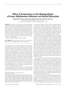
The plot in Figure 1 illustrates the rate of toluene degradation with increase in time. It is seen that increase in time yield decrease in toluene concentration. The variation in toluene concentration can be attributed to variation in time as well as the physicochemical parameter. The micro-organisms within 3 h degraded significant amount of substrate. However, the rate of degradation soon started declining from the 5th h. This lasted for about five hours. The degradation soon stopped after the 11th h. In the microbial population plot depicted in Figure 2, the microbes experienced lag for about 4 h. This was followed by an accelerated growth rate, which lasted for 2.5 h. Their growth became static from the 8th hour, which lasted for two hours. They began to die from the 10th h. Line weaver-Burk plot has been constructed below in Figure 3 in order to derive the various parameters for the Michaelis-Menten equation. The equation y = mx + c can be derived thus:

It can be seen from Figure 4, the substrate-time plot of phenol that it experienced a period of steady growth for over 20 h. This was soon followed by the steadily decreasing consumption of the substrate for about 18 h. In the microbial growth plot depicted in Figure 5, the microbes underwent a lag phase for about 16 h. This was followed by an exponential phase of 20 h. The exponential growth soon declined from the 25th h. Lineweaver-Burk plot has been constructed below, in Figure 6 in order to derive the various parameters for the Michaelis-Menten equation. The equation y = mx + c can be derived thus: y = 8026.7x – 191.94, Slope = 8026.7, 1/Vmax or Intercept c = -191.94, Therefore, Vmax = 0.0053mg/l per h.

Km/Vmax. = 8026.7, Therefore, Km = 41.82mg/l per h.

Ukpaka.

51

Table 4. Isolates of heterotrophic and Petroleum/aromatic hydrocarbon utilizing bacteria.

ISO 1 Rods -

+

-

+

+

+

+

+

+

+

+ + +

+ -

+ + +

+ +

+ + +

+ +

+ + -

+ + -

+ -

-

-

-

+

-

-

-

-

-

-

+

-

-

-

+

+

-

+ +

+ +

+

+

+

+

+

+

+

+

+

+

+

+ +

+ +

+ +

+ +

+ +

+ +

+

+ +

+ +

Raw data for benzene

Raw data for benzene

The plot in Figure 7 depicts the degradation rate of benzene in fresh water; it can be seen from the substrate-time plot of benzene that in about 8.5 h, 23 mg/l of substrate had been consumed. The degradation rate decreased till it stopped completely after 12 h. The degradation plot of benzene is slightly similar to that of toluene. In microbial growth plot depicted in Figure 8, the Microbes underwent lag for about 3 h. This was followed by an exponential phase of 13 h. They began to die out by the 10th h.

The plot in Figure 7 depicts the degradation rate of Benzene in fresh water; it can be seen from the substrate-time plot of Benzene that in about 8.5 h, 23 mg/l of substrate had been consumed. The degradation rate decreased till it stopped completely after 12 h. The Degradation Plot of Benzene is slightly similar to that o f Toluene. In Microbial growth plot depicted in Figure 8, the Microbes underwent lag for about 3 h. This was followed by an exponential phase of 13 h. They began to die out by the 10th h.

Flavo bacterium

ISO 2 Rods -

Chromo bacterium

ISO 3 Rods +

Bacillus sp

ISO 4 Rods -

Escherichia coli

ISO 5 Cocci -

Pseudomonas sp

ISO 6 Rods -

Escherichia coli

ISO 7 Rods -

Pseudomonas sp

+ + -

Possible organism

ISO 8 Cocci +

Streptococcus sp

+

+ + -

ISO 9 Cocci -

Pseudomonas sp

+

+ -

Lactose Sucrose

ISO 10 Rods +

Bacillus sp

+

-

Glucose

ISO 11 Rods -

Chromo bacterium

+

Oxidase Conagulase Mority Methyl red Vooges Prokase

ISO 12 Rods -

Escherichia coli

Catalase

Micrococcus

ISO 13 Cocci +

Total Heterotrophic

Isolate designation Morphology Gram reaction

Line weaver-Burk plot has been constructed, in Figure 9 in order to derive the various parameters for the Michaelis-Menten equation. The Equation y = mx + c can be derived thus: y = 1.973 – 2.685, Slope = 1.973 1/Vmax or Intercept c = - 2.685, Therefore, Vmax = 0.3724mg/l per hour. Km/Vmax. = 1.973, Therefore, Km = 0.7348mg/l per hour.

52

J. Bacteriol. Res.

To luene

4

Substrate conc. (mg/l)

Toluene Conc. (mg/L)

5

3 2 1

0

5

1

1

6 0 5 0

Phenol

4 0 3 0 2 0 1 0

Time (h)

Figure 1. Toluene consumption with respect to time.

0

2 0

4 0

Time (h)

6 0

Figure 4. Phenol degradation plot of substrate concentration versus time for fresh water medium. Microbes Microbial Pop. (cfu/ml)

1200 900

1000

800 Microbial Pop. (Cfu/ml)

800 600 400 200

0

5

1

1

700 600 Microbes

500 400 300 200 100

Time (h)

Figure 2. Microbial growth versus time.

0

2

4

6

Time (h)

Figure 5. Microbial growth versus time for fresh water medium in phenol degradation.

3 y = 157.21x – 6.7076

2.5 2

25

1.5

20

1/v

1/v

30

1 0 0

0.02

0.04

0.06

0.08

1/[S] Figure 3. Line weaver-Burk plot of 1/V versus 1/S for fresh water medium.

y = 8026.7x – 191.94

15 10 5 0 0.024

0.024

0.025

0.025

0.026

0.026

0.027

1/[S]

Conclusion Predicting the rate of degradation of aromatic compounds requires a detailed understanding of the controlling processes and their dependence on some of the

Figure 6. Line weaver-Burk plot of phenol in 1/V versus 1/S.

physicochemical parameters as well as environmental conditions. Simulation results were presented from the

Ukpaka.

50

Benzene

Substrate conc. (mg/l)

45 40 35 30 25 20 15 10

0

5

10

15

Time (h)

Figure 7. Benzene degradation plot of substrate concentration versus time for fresh water medium.

Microbial population (cfu/ml)

1200

1000 800 600 Microbes

400 200

0

5

10

In the evaluation of the rate of degradation of aromatic compounds, the properties of the fresh water medium was considered as a major factors that influence the biodegradation process. The microorganisms used in the investigation were found capable of degradating toluene, benzene and partially phenol. It is considered by the author that the bioremediation or degradation of aromatic compounds e.g toluene, benzene and phenol as presented in this paper can be more effective if inhibiting agents are taking care of. Isolation, identification and characteristics of heterotrophic and petroleum/aromatic hydrocarbon utilizing bacteria was presented in this paper with a view of possible organisms present in system.

Nomenclature

Figure 8. Microbial growth versus time for fresh water medium in benzene degradation

8 y = 1.973x – 2.685

1/v

6 4

2

0 2

model developed with was capable of addressing a wide range of some physicochemical conditions that influence the degradation of toluene, phenol and benzene in a fresh water medium in Niger Delta Area of Nigeria. Our comparison of benzene, toluene and phenol degradation in a fresh water medium under different physicochemical parameters indicates that biodegradation of benzene and toluene was more effective than phenol. The physiochemical parameters play a major role in determining the rate of degradation of aromatic compounds in aqueous medium, since these pavements affect many biochemical processes, both in dry and wet season. The results obtained in this paper were very promising since Pseudomonas putida was able to degrade the aromatic compounds in the fresh water medium. This study has established that:

15

Time (h)

1

53

3

4

Y = Yield coefficient (g/cell/l) ∆X = Change in biomass concentration (mg/l) ∆S = Change in substrate concentration (mg/l) Yx/s = Yield coefficient for biomass (g/cell/l) Yp/s = Yield coefficient for products (g/cell/l) S = Substrate concentration (mg/l) Ya = Yield coefficient for the conversion of feed or substrate into the mass of cells (g/cell/ml). m = Specific requirement for maintenance (mg/l) dS = Change in substrate concentration (mg/l) X = Biomass concentration (mg/l) Rx = The rate of reaction of substrate (mg/l)

dX dt

= Change in biomass concentration per unit time

µ t IS KI

= = = =

5

1/[S]

Figure 9. Line weaver-Burk plot of benzene in 1/V versus 1/S for fresh water medium.

(mg/l/h) Biomass constant or specific growth rate (mg/l) Time (h) -1 Salinity inhibition constant (h ) Substrate inhibition constant (mgl-1)

54

J. Bacteriol. Res.

Constant depending on culture (h-1) Maximum specific growth rate (mg/l) Salinity level (% g/cm3) Density of water medium (g/cm3) Equilibrium constant of substrate (dimensionless) Constant for the salinity inhibition of maximum specific growth rate (h-1) MToT = Total mass of substrate in the liquid phase in the bioreactor (g) or (cm3) Ma = Mass or volume of substrate in the gaseous phase in the bioreactor (g) or (cm3) R = Universal gas constant T = Temperature H = Enthaphy 3 Va = Volume of substrate in gaseous phase (cl ) 3 VL = Volume of substrate in liquid phase (cl ) dP = Change in product concentration (mg/l) δ = Constant of pH dependent (dimensionless) ε = Constant of pH dependent (dimensionless) SL = Substrate in liquid phase (dimensionless) Ai = Positive constant (dimensionless) KI = Positive constant (dimensionless) τ = Cell age (h) (dimensionless) I*S µm Sa ρ KS Da

= = = = = =

REFERENCES Adamczewska M, Siepak J, Gramowska H (2000). Studies of levels of polycyclic aromatic hydrocarbons in soils subjected to antropopressure in the city of Poznafi. Pol. J. Environ., 4: 305. Aksu Z, Gonen F (2004). Biosorption of phenol by immobilized activated sludge in a continuous packed bed: Prediction of breakthrough curves. Process Biochem., 39(5): 599-613. Alexievaa Z, Gerginova M, Zlateva P, Peneva N (2004). Comparison of growth kinetics and phenol metabolizing enzymes of Trichosphoron Cutaneum R57 and mutants with modified degradation abilities. Enzym. Microb. Technol., 34(3-4): 242-247. Annadurai G, Juang RS, Lee DJ (2002). Microbiological degradation of phenol using mixed liquors of Pseudomonas putida and activated sludge. Waste Manag., 22(7): 703-710. Bandhyopadhyay K, Das D, Bhattacharyya P, Maiti BR (2001). Reaction engineering studies on biodegradation of phenol by Pseudomonas putida MTCC 1194 immobilized on calcium alginate. Biochem. Eng. J., 8(3): 179-186. Banerjee G (1997). Treatment of phenolic wastewater in RBC reactor. Water Res., 31(4): 705-714. Belcher R, Nutten AJ, Macdonald AMG (1970). Quantitative Inorganic rd Analysis. 3 edn. London: Burtterworths, p. 47. Buitron G, Gonzalez LM, Lopez-Marin A (1998). Biodegradation of phenolic compounds by an acclimated activated sludge and isolated bacteria. Water Sci. Technol., 37(4-5): 371-378. Chryplewicz-Kalwa M (1999). Characteristic of the rivers in the Wroclaw province in respect of the content of polycyclic aromatic hydrocarbons (in Polish). Gosp. Wodn., 3: 103. Chung TP, Tseng HY, Juang RS (2003). Mass transfer effect and intermediate detection for phenol degradation in immobilized Pseudomonas putida systems. Process Biochem., 38(10): 14971507. Dauta A (1982 ). Conditions de development du phytoplacton. Etude comparative du comportement de huit especes en culture: Role des nutriments, assimilation et stockage intracellulaire. Ann. Limnol., 18(3): 33-40. De Voogt P, Van Hattum PB, Leonards P, Klamer JC, Govers H (1991). Bioconcentration of polycyclic aromatic hydrocarbons in the guppy (Peocillia reticulate). Aquat. Toxicol., 20: 169-194.

Djomo JE, Ferrioer V, Gauthier L, Zoll-Moreux C, Marty J (1995). Amphibian macronucleus test in vivo: Evaluation of the genotoxicity of some polycyclic aromatic hydrocarbons found in a crude oil. Mutagenesis, 10(3): 223-226. Djomo JE, Garrigues P, Narbonne F (1996). Uptake and Depuration of polycyclic aromatic hydrocarbons from sediment by the zebrafish (Brachydanio Rerio). Environ. Toxicol. Chem., 15(7): 1177-1181. Djomo JE, Dauta A, Ferrier V, Narbonne JF. Monkiedje A, Njine T, Garrigues P (2004). Toxic effects of some major polyarmatic hydrocarbons found in crude oil and aquatic sediments on Scenedesmus subspicatus. Water Res., 38: 1817-1821. Egberongbe FOA, Nwilo PC, Badejo OT (2006). ‘Oil Spill Disaster Monitoring along Nigerian Coastline’, Disaster Preparedness and Management: Shaping the Change, Munich, Germanym, pp. 28-34. Eisler R (1987). Polycyclic aromatic hydrocarbon hazards to fish, wildlife, and invertebrates: A synoptic review. US Fish Wildl. Serv. Biol. Rep., 85: 1-11. Gernjak W, Krutzler T, Malato AGS, Caceres J, Bauer AR (2003). Fernandez-Alba, Photo-Fenton Treatment of water containing natural phenolic pollutants. Chemosphere, 50: 71-78. Geyer H, Viswanathan R, Freitag D, Korte F (1981). Relationship between water solubility of organic chemicals and their bioaccumulation by the alga chlorella. Chemosphere, 10(11/12): 1307-1313. Godjevargova T, Ivanova D, Alexieva Z, Dimova N (2003). Biodegradation of toxic organic components from industrial phenol production waste waters by free and immobilized Trichosporon cutaneum R57, Process Biochem., 38(6): 915-920. Gonzalez G, Herrera MG, Garcia MT, Pena MM (2001). Biodegradation of phenol in a continuous process: comparative study of stirred tank and fluidized-bed bioreactors, Bioresour, Technol., 76(3): 245-251. Halsall CJ, Barrie LA, Fellin P, Muir CG, Billeck BN, Lockhartl FYA (1997). Spatial and temporal variation of polycyclic aromatic hydrocarbons in the Arctic atmosphere. Environ. Sci. Technol., 31: 3593. Hao OJ, Kim MH, Seagren EA, Kim H (2002). Kinetics of phenol and chlorophenol utilization by Acinetobacter species. Chemosphere, 46(6): 797-807. Hidalgo A, Jaureguibeitia A, Prieto MB, Fernández CR, Serra JL, Llama MJ (2002). Biological treatment of phenolic industrial wastewaters by Rhodococcus erythropolis UPV-1. Enzyme Microb. Technol., 31(3): 221-226. Hutchinson TC, Hellebust JA, Mackay D, Tam D, Kauss P (1979). Relationship of hydrocarbon solubility to toxicity in algae, cellular membrane effects, In: Oil Spill Conference American Petroleum Institute, Washington, DC, pp. 541-547. IARC (1993). Monograph on the evaluation of carcinogenic risks of chemicals to man: Certain polycyclic hydrocarbons and heterocyclic compounds. Lyon, France, 3: 22-34. Kibret M, Somitsch W, Robra KH (2000). Characterization of a phenol degrading mixed population by enzyme assay. Water Res., 34(4): 1127-1134. Knightes CD, Peters CA (2006). Multisubstrate Biodegradation kinetics for binary and complex mixtures of polycyclic aromatic hydrocarbons. Environ. Toxicol. Chem., 25(7): 1746-1756. Kochany J, Maguire RJ (1991). Abiotic transformations of polynuclear aromatic hydrocarbons and polynuclear aromatic nitrogen heterocycles in aquatic environments. Sc. Total Environ., 144: 17. Kowalczyk D, Swietlik R, Dojlido J (2000). Polycyclic aromatic hydrocarbons in aquatic environment of the Radomka River basin. Field study in Poland. Environ. Prot. Eng., 26(4): 51. th Kreyzig E (1999). Advanced Engineering Mathematics. 8 edn. New York: John Wiley and Sons, Inc., pp.1–21. Kumar A, Kumar S (2004). Biodegradation kinetics of phenol and catechol using Pseudomonas putida MTCC 1194. Biochem. Eng. J., 22: 151-159. Kumaran P, Paruchuri YL (1997). Kinetics of phenol biotransformation. Water Res., 31(1): 11-22. Lante A, Crapisi A, Krastanov A, Spettoli P (2000). Biodegradation of phenols by laccase immobilised in a membrane reactor. Process Biochem., 36(1-2): 51-50. Lee FR, Gardner WS, Anderson JW, Blaylock JW, Barwell-Clarke J

Ukpaka.

(1978). Fate of polycyclic aromatic hydrocarbons in controlled ecosystem enclosures. Environ. Sci. Technol., 7: 832. Lemaire P, Lemaire-Gony S, Berhaut J, Lafaurie M (1992). The uptake, metabolism and biological half-life of benzo(a)pyrene administered by force-feeding in sea bass (Dicentrarchus labrax). Ecotoxicol. Environ. Saf., 23: 244-251. rd Levenspiel O (1999). Chemical Reaction Engineering. 3 edn. New York: John Wiley and Sons, Inc., pp. 611-627. Margesin R, Fonteyne PA, Redl B (2005). Low-temperature biodegradation of high amounts of phenol by Rodococcus spp. And basidiomycetous yeasts. Res. Microbiol., 156(1): 68-75. Marrot B, Barrios MA, Moulin P, Roche N (2006). Biodegradation of high phenol concentration by activated sludge in an immersed membrane bioreactor. Biochem. Eng. J. 30: 174-183. Mekenyan OG, Ankley GT, Veith GD, Call DJ (1994). ASARs for photoinduced: Acute lethality of polycyclic aromatic hydrocarbons to Daphnia magna. Chemosphere, 28(3): 567-582. Mekenyan OG, Ankley GT, Veith GD, Call DJ (1995). QSARs for photoinduced toxicity of aromatic compounds. SAR QSAR Environ. Res., 4: 139-145. Mill T, Babey WR, Lan BY, Baraze A (1981). Photolysis of polycyclic aromatic hydrocarbons in water. Chemosphere, 11/12: 1281. Miller RM, Singer GM, Rosen JD, Bartha R (1988). Photolysis primes biodegradation of benzo(a)pyrene. Appl. Environ. Microbial., 58(5): 1724-1730. Monteiro AMG, Boaventura AR Rodrigues AE (2000). Phenol Biodegradation by Pseudomonas putida DMS 548 in a batch reactor, Biochem. Eng. J., 6(1): 45-49. Mordocco A, Kuek C, Jenkins R (1999). Continuous degradation of phenol at low concentration using immobilized Pseudomonas putida. Enzym. Microb. Technol., 25(6): 530-536. rd Morrison RT, Boyd RN (1974). Organic Chemistry. 3 edn. Boston: Okoh AI (2002) Assessment of the Potentials of some Bacterial Isolates for Application in the Bioremediation of Petroleum Hydrocarbon polluted soil. Ph.D Thesis. Obafemi Awolowo University, Ile-Ife, Nigeria, pp. 7-130. Narbonne JG, Ribera D, Garrigues P, Lafaurie M, Romana A (1992). Different Pathways for the uptake of benzo(a)pyrene adsorbed to sediment by the mussel Mytilus galloprovincialis. Bull. Environ. Contam. Toxicol., 49: 150-156. Neter J, Wasserman W, Kutner MH (1985). Applied linear statistical models. 2nd ed. Homewood, IL: Richard D. Irwin, pp. 171-174. Newsted JL, Giesy JP (1987). Predictive models for photoinduced acute toxicity of polycyclic aromatic hydrocarbons to Daphnia magna Strauss (Cladocera, Crustacea). Environ. Toxicol. Chem., 6: 445461. Nuhoglu A, Yalcin B (2005). Modelling of Phenol Removal in a batch reactor. Process Biochem., 40(3-4): 1233-1239. O’Brien PJ (1991). Molecular mechanisms of quinine cytotoxicity. Chem. Biol. Interact., 80: 1-41. Okoh AI (2006). ‘Biodegradation Alternative in the Cleanup of Petroleum Hydrocarbon Pollutants.’ Biotechnol. Mol. Biol. Rev., 1(2): 38-50. Pai SI, Hsu YL, Chong NM, Sheu CH (1995). Chem. Continuous degradation of phenol by Rhodococus sp. immobilized on granular activated carbon and in calcium alginate. Biorescour. Technol., 51(1): 37-42. Park C, Marchland EA (2006). ‘Modelling Salinity Inhibition Effects During Biodegradation of Perchlorate.’ J. Appl. Microbiol., 101: 222233. Pazarlioglu NK, Telefoncu A (2005). Biodegradation of phenol by Pseudomons putida immobilized on activated pumice particles. Process Biochem., 40: 1807-1814.

55

Prasad R (2000). Petroleum Refining Technology. Nai Sarak Delhi: Khanna Publishers, pp. 346-349. Prieto MB, Hidalgo A, Serra JI, Llama MJ(2002). Degradation of phenol by Rhodococcus crythropolis UPV-1 immobilized on Biolite in a packed-bed reactor. J. Biotechnol., 97: 1-11. Reardon KF, Mosteller DC, Rogers J, DuTeau NM, Kim KH (2002). ‘Biodegradation Kinetics of Aromatic Hydrocarbon Mixtures by Pure and Mixed Bacterial Cultures.’ Environ. Health Perspect., 110(6): 1005-1010. Richardson JF, Peacock DG (19991). “Biochemical Reactors and rd Process Control.’ Coulson and Richardson Chemical Engineering: 3 edn. Linacre House: Butterworth-Heinemann, 3: 330-340. Sa CSA. Boaventura RAR (2001). Biodegradation of phenol by Pseudomonas putida DSM 548 in a trickling bed reactor. Biochem. Eng. J., 9(3): 211-219. Sims RC, Overcash MR (1983). Fate of polynuclear aromatic compounds (PNAs) in soil-plant systems. Residue Rev., 88: 1-68. Suietlik R, Kowalczyk D, Dojlido J (2002). Influence of selected physicochemical factors on the Degradation of PAHs in water. Polish J. Environ. Stud., 11(20): 165-169. Swallow KC, Taghizadeh K, Weakland S, Plummer EF, Bussby WF, Lafleur AL (1995). Photooxidation of selected polycyclic aromatic hydrocarbons in aqueous organic media in the presence of Ti(IV)oxide. Int. J. Environ. Chem., 60: 113. Thomas SD, LI QX (2000). Immunoaffinity chromatography for analysis of polycylic aromatic hydrocarbons in corals. Environ. Sci. Technol., 34: 2649. Timur S, Pazarlioglu N, Piloton R Telefoncu A (2003). Detection of phenolic compounds by thick film sensors based on Pseudomonas putida. Talanta, 61(2): 87-93. Ukpaka CP (2010). Investigation into the Rain Water quality of Ogba Community in Niger Delta Area of Nigeria. The Nigerian Academic Forum: Multidiscip. J., 18(2): 1-11. Ukpaka CP (2004). Comparative Impact of Drilling Mud and Drill Cuttings on the Environment. Int. J. Sci. Tech. Nig., 2(3): 38-41. Ukpaka CP (2004). Development of Model for Crude Oil Degradation in a Simplified Stream System. Int. J. Sci. Technol., 3(2): 34-37. Ukpaka CP (2005). Biodegradation Kinetics for the production of carbon dioxide from natural aquatic ecosystem polluted with crude oil. J. Sci. Technol. Res., 4(3): 41-49. Vysotskaya NA, Bortun LN (1984). The mechanism of radiation-induced hemolytic substitution of condensed aromatic hydrocarbons in aqueous solutions. Rad. Phys. Chem., 23(6): 731-738. Wang SJ, Loh KC (1999). Modelling the role of metabolic intermediates in kinetics of phenol biodegradation. Enzym. Microb. Technol., 25: 177-184. Watanabe K, Hino S, Takahashi N (1996). Responses of activated sludge to an increase in phenol loading. J. Ferment. Bioeng., 82(5): 522-524. Zepp RG, Hoigne J, Bader H (1987). Nitrate-induced photooxidation of trace organic-chemical in water. Environ. Sci. Technol., 21(5): 443450. Zerbe J, Elbanowska H, Siepak J, Sobczynski T, Kabacinski M, Gramowska HH (1994). Metals and polycyclic aromatic hydrocarbons in the lakes water of the Wielkopolski National Park (In polish). Gosp. Wodn., 8: 174. Zhu X, Venosa AD, Suidan MT, Lee K (2001). ‘Guidelines for the Bioremediation of Marine Shorelines and Fresh Water Wetlands.’ U.S. Environmental Protection Agency, Contract 68-c7-0057, pp. 1163.