Chalmers Publication Library Biologically inspired algorithms applied to prosthetic control
This document has been downloaded from Chalmers Publication Library (CPL). It is the author´s version of a work that was accepted for publication in: BioMed 2012 , February 15 – 17, 2012, Innsbruck, Austria
Citation for the published paper: Ortiz-Catalan, M. ; Brånemark, R. ; Håkansson, B. (2012) "Biologically inspired algorithms applied to prosthetic control". BioMed 2012 , February 15 – 17, 2012, Innsbruck, Austria(track 764), pp. 035. http://dx.doi.org/10.2316/P.2012.764-035 Downloaded from: http://publications.lib.chalmers.se/publication/162938
Notice: Changes introduced as a result of publishing processes such as copy-editing and formatting may not be reflected in this document. For a definitive version of this work, please refer to the published source. Please note that access to the published version might require a subscription.
Chalmers Publication Library (CPL) offers the possibility of retrieving research publications produced at Chalmers University of Technology. It covers all types of publications: articles, dissertations, licentiate theses, masters theses, conference papers, reports etc. Since 2006 it is the official tool for Chalmers official publication statistics. To ensure that Chalmers research results are disseminated as widely as possible, an Open Access Policy has been adopted. The CPL service is administrated and maintained by Chalmers Library.
(article starts on next page)
BIOLOGICALLY INSPIRED ALGORITHMS APPLIED TO PROSTHETIC CONTROL Max Ortiz-Catalan *, ** * Department of Signals and Systems, Biomedical Engineering Division, Chalmers University of Technology Gothenburg, Sweden email:
[email protected] ABSTRACT Biologically inspired algorithms were used in this work to approach different components of pattern recognition applied to the control of robotic prosthetics. In order to contribute with a different training paradigm, Evolutionary (EA) and Particle Swarm Optimization (PSO) algorithms were used to train an Artificial Neural Network (ANN). Since the optimal input set of signal features is yet unknown, a Genetic Algorithm (GA) was used to approach this problem. The training length and rate of convergence were considered in the search of an optimal set of signal features, as well as for the optimal time window length. The ANN proved to be an accurate pattern recognition algorithm predicting 10 movements with over 95% accuracy. Moreover, new combinations of signal features with higher convergence rates than the commonly found in the literature were discovered by the GA. It was also found that the PSO had better performance that the EA as a training algorithm but worse than the well established Back-propagation. The latter considered accuracy, training length and convergence. Finally, the common practice of using 200 ms time window was found to be sufficient for producing acceptable accuracies while remaining short enough for a real-time control. KEY WORDS Pattern Recognition, Rehabilitation Engineering, Biomechatronics, Biomedical Signal Processing
1
Introduction
The lack of classification algorithms [1] and control systems [2] were once the principal issues for complex prosthetic control. Nowadays several researchers have shown the possibility to identify finger and hand positioning using a variety of pattern recognition (PatRec) algorithms such as: • Artificial neural networks (ANNs) [2–6]. • Support vector machines (SVM) [7, 8]. • Gaussian mixture models (GMMs) [9]. • Discrete wavelet transform (Wavelets) [10].
Rickard Br˚anemark ** and Bo H˚akansson * ** Centre of Orthopeadic Osseointegration, Dept. Orthopedics, Sahlgrenska University Hospital, Gothenburg University, Gothenburg, Sweden • Hidden Markov models (HMM) [11]. • Fuzzy logic [12]. • Linear discriminant analysis (LDA) [13]. Manipulation of different devices like robotic arms using Myoelectric Signals (MES) as information sources and SVM as control algorithm has been proved to be a feasible technology [7]. In patients where myoelectric control is not possible, EEG in combination with ANNs have been used instead [4]. These studies have demonstrated the identification of several degrees of freedom (DoF) which would be a significant improvement over the current myoelectric prostheses that rarely control 2 DoF simultaneously. However, they have all been short-term implementations and despite the extensive work done in this field, there is still not a generalized agreement in the optimal way to conduct PatRec, nor the optimal way to record MES that allows for a long-term implementation. Therefore, there is a need to continue research in this area to overcome the issues of a long-term stable and robust implementation of PatRec based prosthetic control. Currently most PatRec algorithms have reached accuracies around 95% and although these studies are difficult to compare because they use different evaluation methodologies, some authors have used just a few of these algorithms in the same system [8, 14, 15]. Hargrove et al suggested that most of the modern algorithms (ANNs-MLP, ANNs-LP, LDA, GMM, HMM) have reached a steady state, where all have similar performance [14]. Therefore we considered important to also explore the signal features used as input of the PatRec besides implementing alternative training paradigms. Different PatRec algorithms have used different signal features from the time and frequency domains. Features such as autoregression coefficients [15,16], mean and median frequency [17], variance and moments [18], etc. The most common features found in the literature, although in different combinations, are mean absolute value, zero crossing, slope sign change, wavelength and root mean square (RMS) [3, 8, 13, 15, 16, 18–22]. Because there is no consensus on which signal features provides a better pattern generalization, 21 features
were explored during this study (Table 1). Some of these characteristics were taken from previous publications and others were selected as typical statistical descriptors. 1 2 3 4 5 6 7 8 9 10 11 12 13 14 15 16
Time Mean Mean absolute Median Mode Standard dev. Variance Wavelength Root mean square Zero crossing Peaks ≥ RMS Peaks mean Peaks mean vel. Slope changes Covariance Correlation Power
(tmn) (tmabs) (tmd) (tmod) (tstd ) (tvar) (twl) (trms) (tzc) (tpks) (tmpks) (tmvel) (tslpch) (cr) (vr) (tPwr)
17 18 19 20 21
Frequency Wavelength Wavelength ranking Mean frequency Median frequency Mean frequency of max(peak) peaks ≥ 2
(fwl) (fwlr) (fmn) (fmd) (fpm)
Table 1. EMG signal features from time and frequency domains used by the Genetic Algorithm in order to find an optimal set for pattern recognition.
Important factors when using PatRec algorithms that are not normally discussed in the literature are the training length and rate of convergence. The former relates to the training time and the latter to how the training algorithm will perform with different subjects. Unlike the rate of convergence, the training length depends heavily on the chosen programming language and hardware where the PatRec training algorithm is executed. It is therefore more critical algorithm-wise to have a higher convergence rate since this will assure that the PatRec training algorithm can be used in more subjects while consuming the same training time. Both the training length and the rate of convergence are monitored during all the experiments in this study. 1.1
Algorithms
ANNs have been widely used in problems characterized by the lack of physical or statistical understanding, statistical variations in the observable data and non-linear mechanism responsible for the generation of the data [23]. Myoelectric signals have been described as a non-stationary stochastic process with approximately zero mean and varying variance [8, 18], or simply as stochastic signals [17, 24] that inherently posses the same characteristics. ANNs are thus chosen in this work as the PatRec algorithm for the identification of isometric movements using EMG. The main drawback of ANNs is that there are no clearly defined rules for designing an optimal network. For instance, the number of neurons in the hidden layer as well as the number of hidden layers play an important role in the network performance. Too few neurons will be equivalent to a brain dead system where the network will not be able to learn the required task. On the other hand, too many neurons are easily over trained, resulting in memorization rather than learning and subsequent loss of generalization. However, from these
scenarios it is always better to have more neurons followed by optimization. The optimal number of neurons, training length, and training data quality are the keys for a good generalization method. Unlike previous studies, the ANNs were trained via two stochastic algorithms, an Evolutionary Algorithm (EA) and Particle Swarm Optimization (PSO), plus Backpropagation (BP) for benchmarking. This decision was made in order to investigate a novel approach to the training problem with proper benchmarking against a well established technique. PSO and EA are artificial intelligence alternatives to purely mathematical optimization algorithms. Its stochastic nature could avoid local optimum that deterministic mathematical algorithms would have normally difficulties to overcome.
2 2.1
Methods Data Acquisition
The recordings were obtained using 8 stainless steel electrodes in a bipolar configuration (4 bipolar electrode pairs), 1 cm diameter and 2 cm inter-electrode distance. Several investigations suggests at least 4 bipolar electrodes are necessary to reach an acceptable degree of signal classification [14, 16, 25]. The position of the electrodes differed from subject to subject and no special consideration on their location was made aside from maintaining approximately the same distance between bipolar pairs in order to cover the entire circumference of the forearm, approximately 5 cm distal to the elbow, one proximal and one distal. This arrangement resulted in 2 bipolar electrodes placed in the flexor side and the other 2 in the extensor side. The lack of selective electrodes placement helps to ensure that the development of the algorithms occurs with extremely low dependency on electrode location, a critical factor to facilitate the fitting of prostheses in the clinic. The in-house designed Bio-amps had over 120 dB of Common Mode Rejection Ratio, a gain of 82 000 and a 1st order Butterworth band-pass filter with cut-off frequencies at 70 and 3 000 Hz. The signal was filtered again digitally with a Butterworth band-stop filter for the power line and harmonic interference (PLH). The signals were sampled at 8 kHz. Patient safety is commonly assured with an isolation stage that prevents counter-current from flowing and discharging on the patient. An isolation amplifier was used in this experiment together with a 1 MΩ resistor in series with the leads to limit the current that could flow to the patient. Special attention must be paid when selecting this resistor as it, in conjunction with the input capacitance of the Inamp, acts as a low-pass filter that can significantly reduce the bandwidth of the system.
2.2
EMG acquisition, processing and patterns
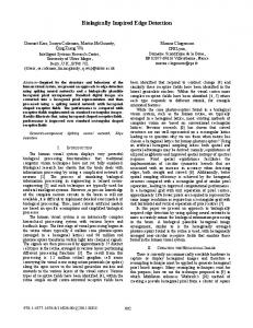
A recording session consisted of Ne different exercises or patterns that were repeated Nr times. These exercises were isometric contractions held for Tc seconds followed by Tr seconds of relaxation time. A percentage of the contraction time (Pct) was established in order to eliminate transient periods. All channels were recorded at a given sampling frequency (Fs ) and digitally combined into 3 matrices containing independent samples to generate training, validation and testing sets. The testing set was used exclusively to measure the accuracy of the network once the training is finished and was therefore not included in the learning process. This differs from standard ANN accuracy reporting but it was considered a more realistic evaluation since this set is independent of the training. In this way, all accuracies reported in this study correspond exclusively to the independent testing set. Accuracy herein is defined as the percentage of correctly registered individual neuron outputs over the total number of outputs. The total number of outputs is given by the number of patterns times the size of testing set. This means that for a given movement not only is the correct number of neuron firings checked, but it is also accounted for whether the others do or do not fire. Ten different finger and hand positions of clinical relevance were recorded and are shown in Figure 1 These were hand open, hand close, hand flexion, hand extension, forearm pronation, forearm supination, side grip, precision grip, thumb up and index pointing. This was the order followed for the subjects to execute each movement per recording session. Most of these movements are considered as featured grip patterns in all known commercial articulated robotic hands, although patients cannot naturally execute them. The currently available, “i-LIMB” (Touch Bionics Inc., UK), and the “VincentHand” (Vincent Systems GmbH, Germany) are capable of performing 6 of these patterns. The “Michelangelo” (Otto Bock, Germany) considers all the movements but lacks actuators for flexion/extension and pronation/supination. Finally, “Bebionic” (RSLSteeper, UK) will provide actuators for all mentioned movements as part of their grip repertoire. 2.3
PSO and EA for ANNs Training
Multi layer perceptron (MLP) [8], Kohonen self-organized map (SOM) [26] and adaptive logic networks (ALN) [27] have reported satisfactory results in similar research. The former and the simplest ANNs architecture, Single layer perceptron (SLP), were chosen as the initial ANN topologies for these experiments. The networks were trained using the mean square error as a fitness measure and all the training algorithms share the same ANN evaluation routines. The training length is an important fact to consider since shorter times favor practical implementations. Al-
Figure 1. The pattern recognition was performed using surface EMG recording of 10 isotonic contractions. These were: hand open (a), hand close (b), hand flexion (c), hand extension (d), forearm pronation (e), forearm supination (f), side grip (g), precision grip (h), thumb up (i) and index pointing (j). These movements were considered of clinical relevance and constitute a major part of the grips repertoire of most commercial articulated robotic hands.
though the algorithms have different methods for searching optima, an objective method to compare the training length is to measure the number of ANN evaluations since all the training algorithms share the same evaluation routine. The number of evaluations is directly related to the number of trainings and is different between each algorithm. If the training algorithm can not converge in a predefined number of trainings, it is marked as a failure. In order to prevent the training algorithms from getting stuck in a non-optimal local minimum, the training was restarted if the validation set had a constant fitness for a given number of trainings after a reset threshold. The information to form the training, validation and testing sets was randomly assigned before each training session or simulation in order to account for stochasticity of the training and to increase the number of trials from a necessarily finite set of measurement data. For example, a set that was used for validation during a given training was used for training or testing in a subsequent trial. Finally the results of all the simulations were averaged. A simulation thus consisted of several trainings iterations until learning is achieved or failure occurs. PSO and EAs are well-established optimization algorithms. The capability of an ANN to produce desired outputs depend on the weight assigned to its connections and the connections themselves. Since the ANN structures were chosen as SLP and MLP, the optimization problem resides exclusively in finding the best weights. Each weight is considered as a variable to be optimized by the PSO and EA. After experimental trials of different parameters, the best performance was obtained by using the configurations shown in Tables 2 and 3 respectively. A detailed description for the implementation of these algorithms can be found in [28]. 2.4
Time Window
The recording time window (TW) required for pattern recognition is another parameter not standardized in the literature. Intuitively, a long recording window will reduce
noise and improve recognition, but it will also slow down real-time control. Surface recordings from 9 different subjects (5 male, 4 female) with average age of 25.4 (min: 22, max: 29, std: 2.3) were used to investigate the effect of reducing the time window. At the same time, the PSO and back-propagation algorithm were compared. The heuristic used to stop the training was to achieve a 100% accuracy of the validation set or a fitness value smaller than 0.1 in the training set when no progress was observed in the fitness of the validation set. The simulation was repeated 100 times for each time window selecting subjects randomly for each simulation. The sets were randomized before each simulation. The set up is presented in Table 4. The ANN used was a SLP with 3 times more neurons in the hidden layer than the number of inputs. Sixteen inputs correspond to 4 channels using 4 of the most popular signal features: mean absolute value, wavelength, zero crossing and RMS. It was experimentally discovered that eliminating normalization improved PSO convergence. Movements were recorded from 10 repetitions of 2 seconds each using a Pct of 50%. Since the number of sets depends on the time window, the training and validation set were fixed at 6 and 2 respectively. The remaining sets were used for testing, i.e. for TW equal to 1 s, the number of testing sets was 2 and for a TW of 0.02 s there were 492 testing sets.
3
Optimization of Signal Features Using an Genetic Algorithm
Since some signal features produce similar characterization and are probably redundant, an EA was used to find the optimal combination. Optimal herein is defined as the features that allow the fastest training with the most accurate prediction and lowest rate of failures. A large amount of features will increase the search space for the training algorithms and thereby increase the number of iterations required to find a solution. The fastest training therefore entails finding the smallest number of features that have the highest characterization. The characterization is directly related to the accuracy. The number of possible combinations of 21 characteristics considering groups from 1 to 21 is around 2 million which is the search space for this problem. Parameter Particles: Maximum velocity: δ t: α: Social component: Cognitive component: Craziness probability: Inertial weight (w): β for inertial weight:
Value 20 20 (±10) 1 1 2 2 0.05 1.4 0.9
Table 2. Summary of the PSO parameters used to train the ANN.
A Genetic Algorithm was the type of EA used in this problem because the coding of the genes as a binary string was straight forward. The activation or deactivation of a chromosome then represents the use of a given signal feature. Since the algorithm used to train the ANNs was stochastic, the EA ran 10 trainings to generate an average of the fitness. The training fitness (ft ) for each algorithm is given by Eq. 1. ft = E ∗ 1/Na ∗ Nf
(1)
where E is the number of evaluations, Na is the accuracy of the ANN and Nf is the fitness of the ANN. As can be deduced from the fitness formula, the EA optimizes by minimizing the fitness. Roulette wheel selection with 80% crossover and 5% mutation rate provide the genetic changes required for evolution. Elitism was used to preserve two copies of the best individual in each generation. A 50-individual population was evolved during 1 000 generations. BP was chosen to train the ANNs mostly for its speed relative to PSO and EA. The training set up for this analysis is summarized in Table 5.
4 4.1
Results EA and PSO for ANNs Training
The EA was considerably slower than the PSO. Traditionally, an EA has a larger population size than PSO and results in more evaluations per generation, and thus slow convergence. The EA population consisted of 50 individuals while PSO had 20 particles. An individual or particle requires at least one evaluation of the fitness measure. Initially, the EA showed poor convergence for more than 2 patterns requiring a large number of generations. Upon scrutiny of the population after no fitness improvement, the execution was easily trapped in local minima with poor diversity as a result. A better performance was reached when the number of copies of the best individual was reduced to one, and a variable mutation rate was introduced. The heuristic for the mutation rate was to increase it if a given percentage of the variances were smaller than the means. The variance is a direct indicator of the spread of the data set and therefore it was considered as a suitable feature. However, due to its poor performance over 4 patterns, even with the latter enhancements, the EA was not investigated further as a PatRec training algorithm. Parameter Individuals: Range Crossover Mutation Tournament selection Inbreeding %
Value 50 ±100 0.8 1/genes 0.75 0.1
Table 3. Summary of the EA parameters used to train the ANN.
0.45
100 Fitness (mean square error)
0.4
Accuracy (%)
95
90
85
80
75
PSO BP 1
0.8
0.6
0.4
0.2 0.1 TW length (s)
0.08
0.06
0.04
0.35 0.3 0.25 0.2 0.15 0.1 PSO BP
0.05 0
0.02
1
0.8
0.6
0.4
0.2 0.1 TW length (s)
0.08
0.06
0.04
0.02
4
14
x 10
1200
12
100
1000
80
10 8 6
Failures (%)
Trainings
Evaluations
800 600
60
40
400 4
PSO BP
2 0
0.8
0.4 0.1 0.06 TW length (s)
PSO BP
200
0.02
0
0.8
0.4 0.1 0.06 TW length (s)
0.02
20
0
PSO BP 1
0.8
0.6
0.4
0.2 0.1 TW length (s)
0.08
0.06
0.04
0.02
Figure 2. These plots show the impact on accuracy, training length and convergence by reduction of the time window length. The comparison between the particle swarm optimization and back-propagation algorithms is also presented in these plots, where the latter proved to have smaller training lengths and a higher rate of convergence.
Parameter Subjects: Age: Male % : Ne : Nr : Tc : Tr : Pct: Normalization: Simulations: Signal features:
Value 9 25.4 ± 2.3 56 4 10 2 2 0.5 No 100 4
Parameter ANN topology: ANN hidden neurons: ANN hiden layers: BP η BP α PSO particles PSO settings Training sets per Ne : Validation sets per Ne : Test sets per Ne :
Value SLP 48 1 0.6 0.1 1012 Tab. 3 6 2 Variable
Table 4. Summary of the settings used in the experiment to investigate the effect of reducing the time window
The PSO showed better convergence than the EA. No major difference in performance was observed with the use of an elite particle or the craziness component. It was discovered experimentally that fitness lower than 0.2 but higher than 0.01 render almost 100% accuracy for 4 patterns (refer to Table 2 for the experimental settings). The PSO algorithm proved to converge 80% faster at identifying less than 5 patterns when compared to the EA. However the convergence was not achieved on 6 patterns with the EA. PSO was unable to classify more than 6 patterns in a reasonable amount of time. However, the BP algorithm showed to have a better performance than both PSO and EA. Figure 2 shows the results of training ANNs with PSO and BP. 4.2
Parameter Time window (ms) Max trainings Reset threshold Ne : Nr : Tc : Tr : Pct:
Value 200 1 000 1 000 10 3 6 6 0.5
Parameter Training sets per Ne : Validation sets per Ne : Test sets per Ne : ANN topology: ANN hidden neurons: ANN hidden layers: BP η BP α
Value 18 9 18 SLP 3 ∗ inputs 1 0.1 0.1
Table 5. Summary of the settings used by the Genetic Algorithm in order to optimize the signal features
Time Window
The effects of reducing the time window are presented in Figure 2. Trend lines are approximately linear for all but the failure rates. A slower convergence for the training algorithms when reducing the time window was expected due to the noise impact increment. Represented in these graphs and also recurrent during the experiments is the observation that as long as it is possible to reach a fitness smaller than 0.1, it would be possible to reach almost 100% of accuracy. 4.3
Signal Features
It was found that although features can produce very similar graphical representation of the same movements (Figure 3), some can be used alone (e.g. tstd, trms, tmabs) while others barely allow any convergence by them selves (e.g. tzc, cv, tvar, twl, fwl, fmn). A consistent result during different runs of the experiment was that no more than 5 features are required to produce an acceptable accuracy.
1.8
1.4 Ch 1 Ch 2 Ch 3 Ch 4
1.2 1
Parameter Subjects: Age: Male % : Ne : Nr : Tc : Tr : P ct: Simulations Normalization: Filtering:
1.4 Ch 1 Ch 2 Ch 3 Ch 4
1.6 1.4
Ch 1 Ch 2 Ch 3 Ch 4
1.2 1
0.6
0.8
1
tstd
trms
tmabs
1.2 0.8
0.8
0.6
0.6 0.4
0.4 0.4
0.2 0 100
0.2
0.2 200
300
400 500 samples
600
300
700
0 100
800
300
400 500 samples
600
12
Ch 1 Ch 2 Ch 3 Ch 4
250
200
0 100
800
200
300
400 500 samples
600
1.4
Ch 1 Ch 2 Ch 3 Ch 4
10
200
700
700
800
Ch 1 Ch 2 Ch 3 Ch 4
1.2 1
Value 200 2 000 1 000 SLP & MLP 3 ∗ inputs 1&2 0.05 0.10 18 9 18
Table 6. Summary of the settings used to validate the sets of features found by the Genetic Algorithm
tvar
fwl
0.8 twl
Parameter Time window (ms) Max trainings Reset threshold ANN topology: ANN hidden neurons: ANN hidden layers: BP η BP α Training sets per Ne : Validation sets per Ne : Test sets per Ne :
8
150
6
0.6 100
4 0.4
50 0 100
Value 11 30.8 ± 12.7 64 10 3 6 6 0.5 110 Yes PLH
2
200
300
400 500 samples
600
700
800
0 100
0.2
200
300
400 500 samples
600
700
800
0 100
200
300
400 500 samples
600
700
800
GFR
Figure 3. These plots show a graphical representation of two movements using 6 different signal features extracted from 4 channels (4 bipolar electrodes) sampled at 10 kHz. The first part of the plot (180 to 380 samples)corresponds to hand open and the second part (550 to 750 samples)to hand close. Although these signals show similar graphs shapes, only the first row (tmabs, trms and tstd) are useful for pattern recognition since the second row (twl, fwl and tvar) hardly allow convergence using settings from Table 7. Results of using the first row of signal features for pattern recognition are shown in Figure 4.
More than 5 features not only slows down the training but also reduces the possibility of convergence, e.g. 21 features produced 100% failures using settings in Table 6. The best individuals found were tested for a 10 pattern recognition task using surface recordings from 11 subjects (7 male, 4 female) with average age of 30.8 (min: 22, max: 50, std: 12.7). Experiment settings are summarized in Table 6 and the results are presented in Figure 4. Error-bars show the mean, minimum and maximum of the accuracy and training length. Another way to measure accuracy is to divide the number of correctly predicted patterns over the total number of pattern analyzed, which is obviously a number smaller than the neuron-firing accuracy (Figure 2) but does not necessarily represent the same behavior at different scales. For this experiment both accuracies are shown since there are differences worthy of note, such as the accuracy of KS5. The convergence produced with the feature sets is shown as a failure percentage with error-bars representing the mean (general failure rate, GFR) and standard deviation. The standard deviation was more representative than the minimum and maximum value in this case. Moreover, the percentage of subjects for which no convergence was achieved (relative failure rate, RFR) is also presented. The GFR represents only a part of robustness of the feature set since it does not show what happens with individual subjects, i.e. a given percentage of failures can consist of relatively small contributions from all subjects or large contributions from a few subjects.
NS2b NS3b NS4 RFR NS2b NS3b NS4
SLP KS4 KS5 2.7% -9.1% 20.0% 8.2% 15.5% 3.6%
MLP KS4 KS5 -4.5% -12.7% 13.6% 5.5% 3.6% -4.5%
SLP KS4 KS5 9.1% -% 18.2% 9.1% 9.1% -%
MLP KS4 KS5 9.1% -9.1% 18.2% -% 9.1% -9.1%
Table 7. Summary of the improvements on convergence of the features sets found by the GA versus known sets used in previous studies. The general failure rate (GFR) corresponds to the total number of failures from all the subjects over the number of simulations. The relative failure rate (RFR) corresponds to the number of subjects where convergence was not achieved over the total number of subjects.
The new sets (NS) of signal features {tstd, tmrs} (NS2b), {tstd, fwl, fmd} (NS3b) and {tmabs, fwl, trms, tzc} (NS4) produced the best performance in terms of accuracy, training length, and failure rate. These two sets were compared with known sets (KS) used in other publications: KS4= {tmabs, tzc, tslpch, twl} [13, 21, 22], and KS5= {tmabs, tzc, tslpch, twl, trms} [8] which is also the set with the most common features found in the literature [3, 13, 15, 16, 18–22]. Interestingly, the EA tended to converge strongly to the KS5 as local optima. The improvement of the new sets over the known sets is summarized in Table 7, the best improvement was found with NS3b as it had the lowest rate of failures. KS5 has a lower failure rate than all the other sets aside from NS3b, but only for a MLP and with a wider variability in accuracy. NS3b, on the other hand, appears more stable for both ANN topologies.
5
Discussion
The PatRec accuracy is directly affected by the PatRec algorithm itself, the PatRec training algorithm, the time window used to compute the signal features, the signal features used as inputs of the PatRec algorithm, and the signal acquisition and processing. The first two have been widely investigated but little has been said about the rest. EA
100
Accuracy (%)
95
90
85
80
SLP Neurons Accuracy MLP Neurons Accuracy SLP Patterns Accuracy MLP Patterns Accuracy trms
tmabs
tstd
NS2a
NS2b NS3a Sets of features
NS3b
KS4
NS4
KS5
2000 SLP MLP Trainings
1500
1000
500
0
trms
tmabs
tstd
NS2a
NS2b NS3a Sets of features
NS3b
KS4
NS4
KS5
100 SLP GFR MLP GFR SLP RFR MLP RFR
Failures (%)
80 60 40 20 0
trms
tmabs
tstd
NS2a
NS2b NS3a Sets of features
NS3b
KS4
NS4
KS5
Figure 4. Comparison between new sets (NS) of signal feature optimized by a Genetic Algorithm and known sets (KS) used in previous research. The discovered sets are: NS2a = {tstd, fmn}, NS2b = {tstd, trms}, NS3a = {tambs, fwl, tzc}, NS3b = {tstd, fwl, fmd} and NS4 = {tmabs, fwl, trms, tzc}. The known sets are: KS4 = {tmabs, tzc, tslpch, twl}, and KS5 = {tmabs, tzc, tslpch, twl, trms} which has the most common features found in the literature. Performance of single features is also presented in order to show that high rates of accuracy can be reached compromising convergence. Although accuracy improvement versus known sets is not significant, the new sets show a better rate of convergence which is argued as more suitable for practical implementations. The general failure rate (GFR) corresponds to the total number of failures from all the subjects over the number of simulations. The relative failure rate (RFR) corresponds to the number of subjects where convergence was not achieved over the total number of subjects.
and PSO here were presented as training algorithms and although PSO showed better performance than EA, the traditional algorithm of Back-propagation proved to be more efficient. Since these algorithms work in different ways, their speed of convergence depends on different factors. PSO and EA required a batch of evaluations per individual or particle to perform one training, while BP required a batch of evaluations per training. A batch of evaluations corresponds to evaluation of all training sets. The latter produces Formula 2, which also applies for the EA. EP SO = PP SO ∗ EBP
(2)
where EP SO and PP SO are the evaluations and particles of the PSO respectively, and EBP the evaluations of the back-propagation algorithm. It can be argued that although PSO and EA required more evaluations per training, it is possible that the number of trainings required for convergence is smaller. According to Figure 2, however, this does not appear to be the case. Although EAs and PSO could be used to train ANNs to identify a small number of patterns, their performance was very poor for more complex recognitions. The number of variables to be optimized by an EA or a PSO aiming to train an ANN (SLP with 48 hidden layer neurons)
to recognize 10 patterns using 4 signal features would be 1306. This is a rather large number for common implementations of these algorithms, and might be an indication that they should not be used to perform the whole training but rather to optimize it. Studies to explore this idea will be performed in the future. An interesting phenomena and property of ANNs is their capability to predict results for which they have not been trained. In numerous instances during on-line recognition, correct prediction of combinations of movements was observed (i.e. wrist flexion with hand opening). The capability for simultaneous control will be studied in the continuation of this work. A time window from 100 to 200 ms is commonly found in the literature [15, 16, 20–22]. In this experiment a significant increase in failures occurred for windows smaller than 200 ms indicating it is a suitable length of time. A real-time control experiment using a conventional myoelectric hand where the delay caused for a 200 ms TW was unperceived for the user was performed to evaluate the practicality of using such length. However, the trade-off between accuracy and speed must be considered in each practical implementation since the hardware likely plays a major role. Despite the fact that the failure rate was not explicitly considered in the fitness function used by the Genetic Al-
gorithm, it was able to produce sets of signal features with better convergence rates. This was due to the fact that a failed training would have the maximum number of evaluations and, since it did not converge, the accuracy and fitness of such an ANN would be low. The performance of a set of signal features was quantified via a combination of accuracy, training speed, and failure rate. It is important to maintain a good balance between these 3 factors for a viable implementation. For instance, a high failure rate indicates success with only limited number subjects, even in the presence of high accuracy and fast training. Most of the literature found does not disclose figures for the training length and/or training failures even though both parameters are critical in a clinical enduse environment. Higher accuracies can clearly be reached with longer training times and high training failures but such an implementation is simply impractical. Although insignificant improvement was observed in accuracy when using the new sets of features in place of the most common ones, the failure rate was reduced by approximately 10%. Such an implementation is thus favorable in a clinical environment where patients with varying muscle strengths will be treated. Similar results were found with two different ANN topologies (SLP and MLP), however, it is worty of mention that verification with different PatRec algorithms is required in order to assess if a given set of features is algorithm specific. It was observed that longer trainings are required when using few signal features (Figure 4), which is not surprising if we consider that the ANN is fed with more information about the system. However, this can not be generalized since the training time as well as the other performance indicators will depend on the signal features forming the sets. Several signal features might reduced the training time but it will also slow down the signal processing and thus result in a slower real-time control. In this experiment all the signal features were already available and therefore the signal processing time was not taken into account. It was found that single signal features can produce high accuracy rates for few subjects but hardly converge for others. Upon scrutiny of the raw recordings of subjects with poor convergence, it was found a relatively high level of noise and low amplitude in comparison to the others where convergence for several feature sets was achieved. The reason for this could be a low muscular mass, the position of the electrodes, or any other environmental or methodological factor of the recording session. The latter issues could be resolved and the recording session could simply be repeated, but a low muscular mass is a more difficult problem to solve. It is precisely this kind of situation for which a more descriptive and robust set of features could be considered useful. Intuitively, the use of such a set of features and in conjunction with a carefully executed recording session, would improve the system’s predictions capability and overall robustness.
6
Conclusions
ANNs proved to be a good classification algorithm for this application although EA and PSO did not show any significant advantage over traditional training algorithms. It was also confirmed that the common practice of employing time windows of 200 ms produces acceptable accuracies while remaining short enough for a real-time control of at least 10 movements. Ten movements already exceeds the state-of-art for DoF that are directly controlled by patients with commercial prosthesis. It is widely known that acceptance of myoelectric prostheses is difficult to achieve. A robotic prosthesis that requires high concentration levels from the patients are impractical for daily life. Despite the fact that pattern recognition algorithms and control engineering have been used since the 1980’s to try to achieve a more natural control of artificial limbs, a long-term implementation is sadly still out of reach for amputees. These experiments were part of a research effort with focus on practical implementations. Analyzing different signal features was thus one of the chief considerations in order to reach this objective. Although no major benefits on accuracy were observed with the newly discovered sets of features, the rate of failures was reduced by roughly 10% in comparison to more conventional implementations. Further studies are still required in order to evaluate the new sets during online recognition.
7
Acknowledgments
The author would like to thank to Stewe J¨onsson at the Department of Prosthetic and Orthotics, Sahlgrenska University Hospital, for the useful insights about daily implementations of prosthetics and Justin F. Schneiderman at MedTech West and the Department of Neuroscience and Physiology, University of Gothenburg, for assistance with preparation of the manuscript. This work was partially funded by VINNOVA and Integrum AB.
References [1] C. Lake and J. Miguelez, “Comparative analysis of microprocessors in upper limb prosthetics,” J Prosthet Orthot, vol. 15, no. 2, 2003. [2] F. Sebelius, L. Eriksson, C. Balkenius, and T. Laurell, “Myoelectric control of a computer animated hand: A new concept based on the combined use of a treestructured artificial neural network and a data glove,” J Med Eng Technol, vol. 30, no. 1, pp. 2–10, Jan 2006. [3] F. Sebelius, B. Ros´en, and G. Lundborg, “Refined myoelectric control in below-elbow amputees using artificial neural networks and a data glove,” J Hand Surg, vol. 30A, no. 4, pp. 780–789, Jul 2005.
[4] C. Guger, W. Harkam, C. Hertnaes, and G. Pfurtscheller, “Prosthetic control by an eeg-based brain-computer interface (bci),” In Proc. AAATE 5th European Conference for the Advancement of Assistive Technology, 1999. [5] D. Bergantz and H. Barad, “Neural network control of cybernetic limb prostheses,” 10th Int Conf IEEE EMBS, vol. 3, pp. 1486–1487, 1988.
“Decoding a new neural-machine interface for control of artificial limbs,” J Neurophysiol, vol. 98, pp. 2974– 2982, 2007. [17] J. Hoffer, R. Stein, M. Haugland, T. Sinkjaer, W. Durfee, A. Schwartz, G. Loeb, and C. Kantor, “Neural signals for command control and feedback in functional neuromuscular stimulation: A review,” J Rehabil Res Dev, vol. 33, no. 2, pp. 145–157, April 1996.
[6] L. Niklasson, M. Bod´en, and T. Ziemke, “Neural control of a virtual prosthesis,” International Conference on ANNs, 1998.
[18] G. Saridis and T. Gootee, “Emg pattern analysis and classification for a prosthetic arm,” IEEE Trans Biomed Eng, vol. BME-29, no. 6, pp. 403–412, Jun 1982.
[7] P. Shenoy, K. Miller, B. Crawford, and R. Rao, “Online electromyographic control of a robotic prosthesis,” IEEE Trans Biomed Eng, vol. 55, no. 3, Mar 2008.
[19] B. Hudgins, P. Parker, and R. Scott, “A new strategy for multifunction myoelectric control,” IEEE Trans Biomed Eng, vol. 40, no. 1, January 1993.
[8] M. Oskoei and H. Hu, “Support vector machine-based classification scheme for myoelectric control applied to upper limb,” IEEE Trans Biomed Eng, vol. 55, no. 8, pp. 1956–1965, August 2008.
[20] N. M. Lopez, F. di Sciascio, C. M. Soria, and M. E. Valentinuzzi, “Robust emg sensing system based on data fusion for myoelectric control of a robotic arm,” Biomed Eng Online, vol. 8, no. 5, 2009.
[9] Y. Huang, K. Englehart, B. Hudgins, and A. Chan, “A gaussian mixture model based classification scheme for myoelectric control of powered upper limb prostheses,” IEEE Trans Biomed Eng, vol. 52, no. 11, pp. 1801–1811, November 2005.
[21] H. Huang, P. zhou, G. Li, and T. Kuiken, “Spatial filtering improves emg classifcation accuracy following targeted muscle reinnervation,” Ann Biomed Eng, 2009.
[10] A. Ramakrishnan and R. Sastry, “Wavelet transforms for compound nerve action potential analysis,” Proc RC IEEE-EMBS & 14th BMESI, 1995. [11] A. Chan and K. Englehart, “Continuous myoelectric control for powered prostheses using hidden markov models,” IEEE Trans Biomed Eng, vol. 52, no. 1, pp. 121–124, January 2005. [12] A. Ajiboye and R. Weir, “A heuristic fuzzy logic approach to emg pattern recognition for multifunctional prosthesis control,” IEEE Trans Neural Syst Rehabil Eng, vol. 13, no. 3, pp. 280–291, Sep 2005. [13] K. Englehart and B. Hudgins, “A robust, real-time control scheme for multifunction myoelectric control,” IEEE Trans Biomed Eng, vol. 50, no. 7, July 2003. [14] L. Hargrove, K. Englehart, and B. Hudgins, “A comparison of surface and intramuscular myoelectric signal classification,” IEEE Trans Biomed Eng, vol. 54, no. 5, pp. 847–853, May 2007. [15] H. Huang, T. A. Kuiken, and R. D. Lipschutz, “A strategy for identifying locomotion modes using surface electromyography,” IEEE Trans Rehabil Eng, vol. 56, no. 1, pp. 65–73, Jan 2009. [16] P. Zhou, M. M. Lowery, K. B. Englehart, H. Huang, G. Li, L. Hargrove, J. P. A. Dewald, and T. A. Kuiken,
[22] J. W. Sensinger, B. A. Lock, and T. A. Kuiken, “Adaptive pattern recognition of myoelectric signals: Exploration of conceptual framework and practical algorithms,” IEEE Trans Neural Syst Rehabil Eng, vol. 17, no. 3, Jun 2009. [23] J. Webster, Medical Instrumentation, Application and Design, 3rd ed. Jhon Wiley & Sons, 1998. [24] L. S¨ornmo and P. Laguna, Bioelectrical Signal Processing in Cardiac and Neurological Applications. Elsevier, Academic Press, 2005. [25] T. Farrell and R. Weir, “A comparison of the effects of electrode implantation and targeting on pattern classification accuracy for prosthesis control,” IEEE Trans Biomed Eng, vol. 55, no. 9, pp. 2198–2211, Sep 2008. [26] A. Lopez, A. Ferreira, I. dos Santos, I. Gerv´asio, S. Salomoni, and G. Araujo, “Development of a microcontrolled bioinstrumentation system for active control of leg prostheses,” Proc 30th Int Conf IEEE EMBS, pp. 2393–2396, 2008. [27] D. Popovic, R. Stein, K. Jovanovic, R. Dai, A. Kostov, and W. Armstrong, “Sensory nerve recording for closed-loop control to restore motor functions,” IEEE Trans Biomed Eng, vol. 40, no. 10, pp. 1024–1031, Oct 1993. [28] M. Wahde, Biologically Inspired Optimization Methods: An Introduction. WIT press, 2008.