ABSTRACT. We present a novel bit rate model for H.264/AVC video encoding which is based on the quantization parameter, the frame rate as well as temporal ...
BIT RATE ESTIMATION FOR H.264/AVC VIDEO ENCODING BASED ON TEMPORAL AND SPATIAL ACTIVITIES Christian Lottermann1,3 Alexander Machado1 Damien Schroeder3 2 Yang Peng Eckehard Steinbach3 1
BMW Group, Munich, Germany; 2 Intel Mobile Communications, Neubiberg, Germany 3 Institute for Media Technology, Technische Universit¨at M¨unchen, Munich, Germany
ABSTRACT We present a novel bit rate model for H.264/AVC video encoding which is based on the quantization parameter, the frame rate as well as temporal and spatial activity measures. With the proposed model, it is possible to trade-off the frame rate versus the quantization parameter to achieve a target bit rate. Our model depends on video activity measures that can be easily calculated from the uncompressed video. In our experiments, the model achieves a Pearson correlation of 0.99 and a root-mean-square error of less than 5% with the measured bit rate values, as verified by statistical analysis. Index Terms— Rate model, H.264/AVC, quantization parameter, temporal resolution 1. INTRODUCTION Due to the success of on-demand and live video streaming applications, almost half of today’s internet traffic is caused by video traffic. According to [1], this share will increase to 80% in 2017. This increase will be mainly driven by video delivery over mobile networks due to the enhanced capabilities of modern consumer electronic devices, such as smartphones, tablet PCs and connected vehicles. Different approaches have been developed to adapt the video stream to the dynamically changing transmission rate between the source and the sink [2], such as scalable video codecs and transcoding of a source video. Furthermore, Dynamic Adaptive Streaming over HTTP (DASH) [3] has been recently standardized, where the video is encoded at different target bit rates and split into video segments of a fixed length. The adaptation of the video stream is controlled at the receiver side, where the DASH client adaptively requests segments at a bit rate that matches the current network performance. To meet the target bit rates on the encoder side, the encoding parameters need to be adjusted for each target rate. Most state-ofthe-art rate control algorithms adjust the quantization stepsize at a fixed temporal resolution to achieve the target rate based on models that relate the average bit rate with the quantization stepsize. For instance, the bit rate models applied in the MPEG-4 [4] and H.264 reference encoder [5] are based on modifications of the quantization stepsizes, besides video specific content parameters. However, these bit rate models ignore the influence of frame rate changes on the bit rate which is a second parameter to adjust the rate. The bit rate model proposed in [6] takes both the impact of quantization and frame rate on the bit rate into consideration. The authors extend the metric in [7] with an estimation model of the two video specific parameters based on three content dependent features, which depend
on the motion-estimation scheme and frame difference information of the underlying codec. In this paper, we propose a bit rate model that considers both spatial quality impairments due to a modification of the quantization parameter and temporal quality impairments resulting from a reduction of the frame rate. Our model depends on constant factors and on content dependent parameters that can be calculated directly from the source video. Hence, the model can be used for rate control to automatically trade off spatial and temporal quality to achieve a certain target bit rate. Our model offers some structural similarity to the model proposed in [7]. However, in comparison with [7] our model only relies on two standard video activity measures (temporal and spatial activity) that can easily be calculated from the source video. The content parameters required for the model in [7] are computationally complex and are partially based on the motion estimation scheme of the underlying video codec. To calculate these parameters, the authors use a dedicated codec-dependent pre-processor. We train and validate our model with typical multimedia domain videos with representative temporal and spatial activity values at one spatial resolution. Our metric shows a high rate prediction performance with a similar performance as [7], but at a much reduced complexity. The main advantage of our approach is that the bit rate of a H.264/AVC video can be estimated independently of codec dependent pre-processors which makes it possible to decouple rate controllers from the actual video encoder. The rest of the paper is organized as follows. Section 2 presents our bit rate model with the estimated parameters based on the temporal and spatial activity. We assess the performance of the parameter estimation and the bit rate model in Section 3, while Section 4 concludes this work. 2. BIT RATE MODEL AND PARAMETER ESTIMATION In this section, we describe the estimation of the video bit rate as a function of the video frame rate and the quantization parameter. Furthermore, we propose models to estimate the video specific, contentdependent modeling parameters. For our investigation we follow a similar approach as proposed by Ma et al. [7]. Therefore, we use a bit rate model that separates the influence of spatial and temporal encoding parameters by means of two factors (spatial correction factor (SCF )) and temporal correction factor (T CF )). Furthermore, we use a maximum bit rate (Rmax ) which is the bit rate of the encoded video at the minimum quantization parameter qp,min and the maximum frame rate fmax .
6 150
8 2
10 5
SA
Different from [7], where the content dependent parameters for the three factors are extracted using a codec dependent pre-processor, we use temporal and spatial activity measures extracted from uncompressed source video to estimate the model parameters. Hence, the model is constructed by the product of the three factors: R(qp , f ) = Rmax · SCF (qp , qp,min ) · T CF (f, fmax ) (1)
100
2.1. Model Parameter Estimation
4
First, we describe the stepwise feature selection methodology we apply to model Rmax , SCF and T CF based on the temporal activity (TA) and spatial activity (SA). We use the TA and SA definitions given in [8]: SA = meantime {stdspace [Sobel(Fn )]}
(2)
T A = meantime {stdspace [Fn − Fn.1 ]}
(3)
TA and SA show different correlations with each of the model parameters in (1). Thus, not all parameters can be modeled equally well by these two features. Therefore, we predict the parameters by the iterative generalized linear regression method (GLM) proposed by McCullagh and Nelder [9] with an analysis on the cross validation error (CVE) as the error criterion to select and combine the most suitable features. The CVE is calculated by the mean of the squared difference of the measured and the predicted value. To further enhance the parameter prediction, we add standard functions of TA and SA, such as the logarithm function, and interaction terms of both features. The general GLM to model the target value of y with N different properties is y=
N X N X
ai · f (xi ) + bi,j · f (xi , xj ) + a0
(4)
i=1 j=1
where the weights of the single features ai and the weights of the interaction terms bi,j are calculated by least square non-linear fitting. We apply the stepwise, iterative feature selection and combination approach proposed in [10]. In the first iteration step, the feature that offers the lowest CVE with the target value is selected. In the following iteration round, we combine this feature with a second feature that offers a lower CVE in combination with the first feature. These iteration steps are repeated until the CVE cannot be reduced any further while adding more features to the GLM. We use leave out one cross validation (LOOVC) to train the weights and calculate the CVE for each feature and feature combination to realize generic results that are also valid for videos outside the training set. For the estimation of the required bit rate model parameters, we select a set of six uncompressed training videos in CIF format (352x288) with a frame rate of 30 frames per second [11]: Akiyo (1), Container (2), Football (3), Foreman (4), Hall (5) and Mobile (6). We select 120 frames of each sequence with stable TA and SA conditions to achieve reliable results. The TA and SA values of the uncompressed videos are displayed in Fig. 1. For each video we create processed video sequences (PVS) by temporally downsampling each video at four different frame rates (15 fps, 10 fps, 5 fps, 3 fps) and different quantization parameters ranging from 24 to 45 with a stepsize of 1. All PVS are encoded in H.264/AVC baseline using x264 [12] with a group-of-pictures (GOP) structure of IPP...P. We use different GOP lengths for each frame rate, such that one GOP has a length of one second. These GOP lengths are applied in typical DASH deployments where the segments usually have an integer length in seconds.
3
9 1 7
50 0
5
10
15
20
25
30
35
TA
Fig. 1: SA/TA values for the training set ( ) and validation set ( ). 2.2. Maximum Rate Parameter Estimation We apply the previously introduced iterative GLM with an analysis on the cross validation error to select the most suitable features to model Rmax . In Table 1 we show the Pearson correlation (PC) and CVE of a selection of features that offer the lowest CVE with the measured Rmax value. At the first iteration step, the interaction term T A · SA offers the lowest CVE of 42273.4 for a single feature and qualifies for the next iteration round. To further improve the estimation performance, we combine this feature with the remaining other features. However, the CVE cannot be reduced any further while adding more features. Therefore, the linear combination for the estimated Rmax depending on SA and TA (marked with st in the following) that offers the lowest CVE is constructed by a single feature and can be written as Rmax,st = ρ1 · T A · SA + ρ0
(5)
with a term depending on the interaction of the product of TA and SA and a constant offset. The values for the model parameters are ρ1 = 0.8149 kbit/s and ρ0 = 139.4017 kbit/s, as determined by least square non-linear fitting. #Iteration
Features
PC
CVE
1
TA SA log(T A) log(SA) T A · SA log(T A · SA)
0.8969 0.5897 0.8687 0.5436 0.9950 0.9263
782079.7 2327440.5 641711.2 2199012.4 42273.4 527599.1
Table 1: Cross-validation results for Rmax values.
2.3. Spatial Correction Factor Estimation The spatial correction factor describes the reduction of the bit rate as a function of the quantization parameter. Fig. 2 shows the video bit rate normalized by the measured Rmax of each individual video as a function of the quantization parameter qp . We derive that the factor should be equal to 1 at qp,min and reduce to 0 for large qp levels. Similar to [7] we use an inverse power function to model the SCF : � SCF (qp , qp,min ) =
qp qp,min
�−a (6)
1
0.8
0.8 T CF (f, fmax )
SCF (qp , qp,min )
1
0.6 0.4 0.2 0
0.6 0.4 0.2
25
30
35
40
0
45
0
5
10
qp
15
20
25
30
f [fps]
Fig. 2: Measured SCF (dots) and estimated SCF (lines) of Eq. 6 for videos of the training set: 1 ( , ), 2 ( , ), 3 ( , ), 4(, ), 5 ( , ), 6 ( , ).
Fig. 3: Measured T CF (dots) and estimated T CF (lines) of Eq. 8 for videos of the training set: 1 ( , ), 2 ( , ), 3 ( , ), 4(, ), 5 ( , ), 6 ( , ).
where a is a content dependent model parameter which specifies how fast the SCF decreases when the quantization parameter increases. We obtain the parameter a for each video by least-square non-linear fitting with the measured values. To estimate a of the SCF based on TA and SA, we follow the same procedure as for the Rmax estimation. In Table 2 the estimation performance for a selection of different features offering the lowest CVE and feature combinations for the different iteration steps are listed. At the first iteration step the feature log(SA) offers the lowest CVE of 0.5139. At the second iteration step, we combine this feature with the other available features. The CVE of the combination of the features T A · SA and log(SA) offers the lowest CVE of 0.0976. Additional iteration steps that take even more features into consideration do not reduce the CVE any further. Hence, we stop the GLM after the second iteration. Based on the results of the performed GLM, the factor a can be estimated as
For the estimation of the content dependent parameter b of the T CF based on TA and SA, we again apply the GLM with an analysis on the CVE. Table 3 shows the estimation performance for a selection of features offering the lowest CVE with the measured values are shown. At the first iteration step, the feature log(T A · SA) offers the lowest CVE with parameter b. However, further GLM iteration steps do not decrease the CVE value. Therefore, we stop the GLM after the first iteration. The SA and TA based model of the b parameter is given by
ast = α2 · log(SA) + α1 · T A · SA + α0
(7)
where the values of the model parameters are given by α2 = 2.0129, α1 = −0.0004 and α0 = −4.6158. #Iteration
1
2
Features
PC
CVE
TA SA log(T A) log(SA) T A · SA log(T A · SA) log(SA),T A · SA
0.5457 0.5685 0.4339 0.6272 0.2600 0.1900 0.9572
0.5391 0.7405 0.6691 0.5139 0.8548 0.7963 0.0976
Table 2: Cross-validation results for SCF values. 2.4. Temporal Correction Factor Estimation Similar as the SCF , the T CF describes the influence of frame rate modifications on the bit rate. Fig. 3 shows the bit rate normalized by Rmax for different frame rates. The factor should be equal to 0 at a frame rate of 0 and increase to 1 for the maximum frame rate. As in [7] we use a power function to model the T CF � �b f (8) T CF (f, fmax ) = fmax where b is a content dependent model parameter which specifies how fast the T CF increases when the frame rate increases.
bst = β1 · log(T A · SA) + β0
(9)
where the weight of the single feature is β1 = 0.1334 and the offset β0 = −0.3072. #Iteration
Features
PC
CVE
1
TA SA log(T A) log(SA) T A · SA log(T A · SA)
0.7607 0.4640 0.8530 0.4746 0.7751 0.8915
0.0222 0.0393 0.0119 0.0401 0.0238 0.0081
Table 3: Cross-validation results for T CF values. 2.5. Spatio-Temporal Rate Model We now integrate the three TA and SA dependent parameters Rmax , SCF and T CF into the overall bit rate model of Eq. 1. Hence, our spatio-temporal rate model (STRM) can be written as � �−ast � �bst qp f ST RM (T A, SA) = Rmax,st · · (10) qp,min fmax where all model parameters are only depending on standard video activity measures of the source video. 3. ASSESSMENT OF THE PROPOSED MODEL In this section, we evaluate the performance of the model parameter estimation and the overall bit rate model. To verify the robustness of the bit rate model also for videos outside the training video set, we use a second set of four validation videos [11]: Mother & Daughter (7), Paris (8), Silent (9) and Deadline (10), temporally and spatially downsampled at the same levels as the training set. The corresponding TA and SA values are displayed in Fig. 1. Finally, we compare the bit rate estimation accuracy of STRM with the bit rate
Measured Rate [kbit/s]
(a) Video 7
(c) Video 9
(b) Video 8
(d) Video 10
1,500
400
800
600
300
600
1,000
400
200
400 500
200
100 0
0
100
200
300
0
400
0
500
1,000
1,500
0
200
0
200
400
600
0
0
200
400
600
800
Estimated Rate [kbit/s]
Fig. 4: Performance evaluation of the rate model for different quantization stepsizes at 30fps ( ), 15fps ( ), 10fps ( ), 5fps ( ) and 3fps ( ). model proposed by Ma et. al [7] (referred to as Ma in the following). 3.1. Maximum Bit Rate Estimation We calculate the PC and RMSE between the measured and estimated Rmax values for the validation video set. The results in Table 4 show a high PC of 0.9888 and a RMSE of less than 161.2 kbit/s for the validation video set which emphasizes the robustness of the model for videos outside the training set. Furthermore, we also determine the performance of the estimation for the training video set and all videos combined. In both cases the performance is at a high level with a PC of larger than 0.99 and a RMSE of lower than 133.5 kbit/s.
PC RMSE [kbits/s]
Training set
Validation set
All videos
0.9950 111.2
0.9888 161.2
0.9912 133.5
Table 4: Rmax estimation performance. 3.2. Spatial and Temporal Correction Factor Estimation Similar to the Rmax performance assessment, we calculate the PC and RMSE between the determined parameter a of the spatial correction factor and the parameter prediction in Eq. 7 with the videos of the training set. The results show a PC of 0.9551 and a RMSE of 0.1780. We also calculate the estimation performance of the b parameter of the temporal correction factor between the determined and estimated values calculated in Eq. 9. The results show a PC of 0.8915 and a RMSE of 0.0712 with the training video set. 3.3. Bit Rate Estimation Performance Finally, we determine the overall performance of the STRM which is based on the TA and SA values only and compare it with the estimation performance of Ma’s bit rate model in [7]. The metric coefficients of Ma are trained with the training video set by least-square non-linear fitting with the measured data based on the content features used in [7]. In Table 5 the statistical measures PC and RMSE normalized by Rmax of both bit rate models for the validation video set are listed. The models are trained with the videos from the training video set only. Both bit rate estimation models achieve a high bit rate prediction performance with a PC of almost 0.99. However, besides the advantages discussed in Section 1, STRM offers an about 6% lower RMSE compared to Ma’s model. The main reason is that Ma’s model does not take modifications of the GOP length for temporally downsampled sequences into consideration, since it has
been developed for GOP structures of a fixed length of 16 frames. A graphical representation of the performance of our proposed STRM with the validation video set is given in Fig. 4 where the relation between predicted and estimated bit rate is displayed for different quantization parameters and frame rates.
Ma[7] STRM
PC
%RMSE
#Parameters
0.9864 0.9898
10.71 4.75
3 2
Table 5: STRM performance comparison of the validation set. To test STRM’s independency of the actual H.264/AVC implementation, we perform a three-way analysis of variance (ANOVA) on the TA and SA values with the H.264/AVC codec-dependent parameters required in [7]. The results show that there is a nonsignificant effect of the codec-dependent parameters and the interaction terms on the TA and SA (p > 0.05), which suggests that STRM is independent of the H.264/AVC implementation. Hence, for the calculation of STRM no codec-dependent pre-processor is required. In this section, we assessed the performance of our proposed STRM for dynamic GOP lengths and achieved a high performance with a PC of 0.99 and a RMSE of less than 5% for the validation video set. We also trained and assessed the performance of the model for fixed GOP lengths and were able to achieve similar performance.
4. CONCLUSION In this paper, we propose a bit rate model for H.264/AVC video encoding which is based on the quantization parameter, frame rate and content dependent video activity measures. Unlike state-of-the-art bit rate models that require a computationally complex pre-processor to estimate the content features from the source video, we use low complexity temporal and spatial activity values that can easily be calculated. Hence, the developed low-complexity bit rate model is more suitable for a real-time estimation of the bit rate. Our proposed STRM offers a PC of 0.99 and a RMSE of less than 5% with the measured bit rate values. In future work, we plan to investigate the influence of the GOP length and structure and other spatial resolutions, such as 1080p, on the bit rate to further enhance the bit rate model. Furthermore, based on STRM and subjective video quality metrics, we intend to develop a rate control scheme based on TA and SA for modifications of the frame rate and quantization parameter.
5. REFERENCES [1] Cisco, “Cisco visual networking index: Forecast and methodology, 2012-2017,” 2013. [2] L. De Cicco, S. Mascolo, and V. Palmisano, “Feedback control for adaptive live video streaming,” in Proceedings of the Second Annual ACM Conference on Multimedia Systems, New York, NY, USA, 2011, MMSys ’11, pp. 145–156, ACM. [3] T. Stockhammer, “Dynamic adaptive streaming over HTTP: Standards and design principles,” in Proceedings of the Second Annual ACM Conference on Multimedia Systems, New York, NY, USA, 2011, MMSys ’11, pp. 133–144, ACM. [4] T. Chiang, H.-J. Lee, and H. Sun, “An overview of the encoding tools in the MPEG-4 reference software,” in IEEE International Symposium on Circuits and Systems, 2000, vol. 1, pp. 295–298. [5] Y. Liu, Z.G. Li, and Y.C. Soh, “A novel rate control scheme for low delay video communication of H.264/AVC standard,” IEEE Transactions on Circuits and Systems for Video Technology, vol. 17, no. 1, pp. 68–78, 2007. [6] Y. Wang, Z. Ma, and Y.-F. Ou, “Modeling rate and perceptual quality of scalable video as functions of quantization and frame rate and its application in scalable video adaptation,” in 17th International Packet Video Workshop, Seattle, WA, USA, 2009, pp. 1–9. [7] Z. Ma, M. Xu, Y.-F. Ou, and Y. Wang, “Modeling of rate and perceptual quality of compressed video as functions of frame rate and quantization stepsize and its applications,” IEEE Transactions on Circuits and Systems for Video Technology, vol. 22, no. 5, pp. 671–682, 2012. [8] Y. Peng and E. Steinbach, “A novel full-reference video quality metric and its application to wireless video transmission,” in IEEE International Conference on Image Processing (ICIP), Brussels, Belgium, 2011, pp. 2517–2520. [9] P. McCullagh and J. A. Nelder, Generalized Linear Models, Chapman and Hall, New York, 1990. [10] Y.-F. Ou, Z. Ma, T. Liu, and Y. Wang, “Perceptual quality assessment of video considering both frame rate and quantization artifacts,” IEEE Transactions on Circuits and Systems for Video Technology, vol. 21, no. 3, pp. 286–298, 2011. [11] “YUV video sequences,” http://trace.eas.asu.edu/yuv/, Accessed June 01, 2014. [12] VideoLAN, “x264 project,” http://www.videolan.org/developers/x264.html, Accessed June 01, 2014.