Journal of Statistical Software ... Athens Univ. of Economics and Business .... coded to any statistical package offering algorithms fitting generalized linear ...
JSS
Journal of Statistical Software September 2005, Volume 14, Issue 10.
http://www.jstatsoft.org/
Bivariate Poisson and Diagonal Inflated Bivariate Poisson Regression Models in R Dimitris Karlis
Ioannis Ntzoufras
Athens Univ. of Economics and Business
Athens Univ. of Economics and Business
Abstract In this paper we present an R package called bivpois for maximum likelihood estimation of the parameters of bivariate and diagonal inflated bivariate Poisson regression models. An Expectation-Maximization (EM) algorithm is implemented. Inflated models allow for modelling both over-dispersion (or under-dispersion) and negative correlation and thus they are appropriate for a wide range of applications. Extensions of the algorithms for several other models are also discussed. Detailed guidance and implementation on simulated and real data sets using bivpois package is provided.
Keywords: bivariate Poisson distribution, EM algorithm, zero and diagonal inflated models, R functions, multivariate count data.
1. Introduction Bivariate Poisson models are appropriate for modeling paired count data exhibiting correlation. Paired count data arise in a wide context including marketing (number of purchases of different products), epidemiology (incidents of different diseases in a series of districts), accident analysis (number of accidents in a site before and after infrastructure changes), medical research (the number of seizures before and after treatment), sports (the number of goals scored by each one of the two opponent teams in soccer), econometrics (number of voluntary and involuntary job changes), just to name a few. Unfortunately the literature on such models is sparse due to computational problems involved in their implementation. Bivariate Poisson models can be expanded to allow for covariates, extending naturally the univariate Poisson regression setting. Due to the complicated nature of the probability function of the bivariate Poisson distribution, applications are limited. The aim of this paper is to introduce and construct efficient Expectation-Maximization (EM) algorithms for such models including easy-to-use R functions for their implementation. We further extend our methodology to construct inflated versions of the bivariate Poisson model. We propose a model that
2
Bivariate Poisson Regression Models
allows inflation in the diagonal elements of the probability table. Such models are quite useful when, for some reasons, we expect diagonal combinations with higher probabilities than the ones fitted under a bivariate Poisson model. For example, in pre and post treatment studies, the treatment may not have an effect on some specific patients for unknown reasons. Another example arises in sports where, for specific cases, it has been found that the number of draws in a game is larger than those predicted by a simple bivariate Poisson model (Karlis and Ntzoufras 2003). In addition, an interesting property of inflated models is their ability to allow for modeling both correlation between two variables and over-dispersion (or alternatively under-dispersion) of the corresponding marginal distributions. Given their simplicity, such models are quite interesting for practical purposes. The remaining of the paper proceeds as follows: in Section 2 we introduce briefly the bivariate Poisson and the diagonal inflated bivariate Poisson regression models. In Section 3 we provide a detailed description of the R functions. Several illustrative examples (simulated and real) including guidance concerning the fitting of the models can be found in Section 4. Finally, we end up with some concluding remarks in Section 5. Detailed description and presentation of the EM algorithms for maximum likelihood (ML) estimation is provided at the appendix.
2. Models for bivariate Poisson data 2.1. Bivariate Poisson regression models Consider random variables Xκ , κ = 1, 2, 3 which follow independent Poisson distributions with parameters λκ , respectively. Then the random variables X = X1 + X3 and Y = X2 + X3 follow jointly a bivariate Poisson distribution, BP (λ1 , λ2 , λ3 ), with joint probability function −(λ1 +λ2 +λ3 )
fBP (x, y | λ1 , λ2 , λ3 ) = e
λx1 λy2 x! y!
min(x,y)
X i=0
x i
!
y i
!
�
i!
λ3 λ1 λ2
�i
.
(1)
The above bivariate distribution allows for positive dependence between the two random variables. Marginally each random variable follows a Poisson distribution with E(X) = λ1 +λ3 and E(Y ) = λ2 + λ3 . Moreover, COV(X, Y ) = λ3 , and hence λ3 is a measure of dependence between the two random variables. If λ3 = 0 then the two variables are independent and the bivariate Poisson distribution reduces to the product of two independent Poisson distributions (referred as double Poisson distribution). For a comprehensive treatment of the bivariate Poisson distribution and its multivariate extensions the reader can refer to Kocherlakota and Kocherlakota (1992) and Johnson, Kotz, and Balakrishnan (1997). More realistic models can be considered if we model λ1 , λ2 and λ3 using covariates as regressors. In such case, the Bivariate Poisson regression model takes the form (Xi , Yi ) log(λ1i ) log(λ2i ) log(λ3i )
∼ = = =
BP (λ1i , λ2i , λ3i ), w> 1i β 1 , > w2i β 2 , w> 3i β 3 ,
(2)
where i = 1, . . . , n, denotes the observation number, wκi denotes a vector of explanatory variables for the i-th observation used to model λκi and β κ denotes the corresponding vector
Journal of Statistical Software
3
of regression coefficients, κ = 1, 2, 3. The explanatory variables used to model each parameter λκi may not be the same. Usually, we consider models with constant λ3 (no covariates on λ3 ) because such models are easier to interpret. Although assuming a constant covariance term results to models that are easy to interpret, using covariates on λ3 helps us to have more insight regarding the type of influence that a covariate has on each pair of variables. To make this understood recall that the marginal mean for Xi is equal (from (2)) to E(Xi ) = > exp(w> 1i β 1 ) + exp(w 3i β 3 ). If a covariate is present in both w 1 and w 3 , then a considerable part of the influence of this covariate is through the covariance parameter that is common for both X and Y variables. Moreover, such an effect is no longer multiplicative on the marginal mean (additive on the logarithm) but much more complicated (multiplicative on λ1 and λ3 and additive on the marginal mean). Jung and Winkelmann (1993) introduced and implemented bivariate Poisson regression model using a Newton-Raphson procedure. Ho and Singer (2001) and Kocherlakota and Kocherlakota (2001) proposed a generalized least squares and Newton Raphson algorithm for maximizing the log-likelihood respectively. Here we construct an EM algorithm to remedy convergence problems encountered with the Newton Raphson procedure. The algorithm is easily coded to any statistical package offering algorithms fitting generalized linear models (GLM). Here, we provide R functions for implementing the algorithm. Standard errors for the parameters can be calculated using the information matrix provided in Jung and Winkelmann (1993) or using standard bootstrap methods. The latter is quite easy since good initial values are available and the algorithm converges fairly quickly. Finally, Bayesian inference has been implemented by Tsionas (2001) and Karlis and Meligkotsidou (2005).
2.2. Diagonal inflated bivariate Poisson regression models A major drawback of the bivariate Poisson model is its property to model data with positive correlation only. Moreover, since its marginal distributions are Poisson they cannot model over-dispersion/under-dispersion. As a remedy to the above problems, we may consider mixtures of bivariate Poisson models like those of Munkin and Trivedi (1999) and Chib and Winkelmann (2001). However, such models involve difficult computations regarding estimation and can not handle under-dispersion. In this section, we propose diagonal inflated models that are computationally tractable and allow for over-dispersion, (under-dispersion) and negative correlation. The results reported are new apart from a quick comment in Karlis and Ntzoufras (2003) and some special cases treated in Li, Lu, Park, Kim, and Peterson (1999), Dixon and Coles (1997) and Wang, Lee, Yau, and Carrivick (2003). In the univariate setting, inflated models can be constructed by inflating the probabilities of certain values of variable under consideration, X. Among them, zero-inflated models are very popular; see, for example, Lambert (1992), Bohning, Dietz, Schlattmann, Mendonca, and Kirchner (1999). Moreover, package zicounts is available via CRAN which can be used to fit zero inflated models. In the multivariate setting, there are few papers discussing inflated model in bivariate discrete distributions. Such models have been proposed by Dixon and Coles (1997) for modeling soccer games, Li et al. (1999) and Wang et al. (2003) who considered inflation only for the (0,0) cell, Wahlin (2001) who discussed zero-inflated bivariate Poisson models and Gan (2000). We propose a more general model formulation which inflates the probabilities in the diagonal of the probability table. This model is an extension of the simple zero-inflated model which
4
Bivariate Poisson Regression Models
allows only for an excess in (0, 0) cell. We consider, for generality, that the starting model is the bivariate Poisson model. Under this approach a diagonal inflated model is specified by (
fIBP (x, y) =
(1 − p)fBP (x, y | λ1 , λ2 , λ3 ), x 6= y (1 − p)fBP (x, y | λ1 , λ2 , λ3 ) + p fD (x | θ), x = y,
(3)
where fD (x | θ) is the probability function of a discrete distribution D(x; θ) defined on the set {0, 1, 2, . . .} with parameter vector θ. Note that for p = 0 we have the simple bivariate Poisson model defined in the previous section. Diagonal inflated models (3) can be fitted using the EM algorithm provided at the appendix. Useful choices for D(x; θ) can be the Poisson, the geometric or simple discrete distributions denoted by Discrete(J). The geometric distribution might be of great interest since it has mode at zero and decays quickly as one moves away from zero. As Discrete(J) we consider the distribution with probability function (
f (x|θ, J) = where
PJ
x=0 θx
θx 0
for x = 0, 1, . . . , J for x = 6 0, 1, . . . , J
(4)
= 1. If J = 0 then we end up with the zero-inflated model.
Two are the most important and distinctive properties of such models. Firstly, the marginal distributions of a diagonal inflated model are not Poisson distributions, but mixtures of distributions with one Poisson component. Namely the marginal for X is given by fIBP (x) = (1 − p) fPo (x | λ1 + λ3 ) + p fD (x | θ),
(5)
where fPo (x | λ) is the probability function of the Poisson distribution with parameter λ. This can be easily recognized as a 2-finite mixture distribution with two components, the one having a Poisson distribution and the other a fD distribution. For example, if we consider a geometric inflation then the resulting marginal distribution is a 2-finite mixture distribution with one Poisson and one geometric component. Thus the marginal mean is given by E(X) = (1 − p) (λ1 + λ3 ) + p ED (X) where ED (X) denotes the expectation of the distribution D(x; θ). The variance is much more complicated and is given by n
o
VAR(X) = (1 − p) (λ1 + λ3 )2 + (λ1 + λ3 ) + p ED (X 2 ) − {(1 − p) (λ1 + λ3 ) + p ED (X)}2 . Since the marginals are not Poisson distributions, they can be either under-dispersed or overdispersed depending on the choices of D(x; θ). For example, if D(x; θ) is a degenerate at one (that is, Discrete(1) with θ > = (0, 1)) implying inflation only on the (1, 1) cell, then, for λ1 + λ3 = 1 and p = 0.5, the resulting distribution is under-dispersed (variance equal to 0.5 and mean equal to 1). On the other hand, if the inflation distribution has positive probability on more points, for example a geometric or a Poisson distribution, the resulting marginal distribution will be over-dispersed. In the simplest case of zero-inflated models, the marginal distributions are also over-dispersed relative to the simple Poisson distribution. Another important characteristic is that, even if λ3 = 0 (double Poisson distribution), the resulting inflated distribution introduces a degree of dependence between the two variables
Journal of Statistical Software
5
under consideration. In general, the simple bivariate Poisson models has EBP (XY ) = λ3 + (λ1 + λ3 )(λ2 + λ3 ). Thus for an inflated model we obtain COVIBP (X, Y ) =
(1 − p) {λ3 + (λ1 + λ3 )(λ2 + λ3 )} + p ED (X 2 ) −(1 − p)2 (λ1 + λ3 )(λ2 + λ3 ) −(1 − p) p ED (X)(λ1 + λ2 + 2λ3 ) − p2 {ED (X)}2 .
The above formulas are a generalization of simpler case where inflation is imposed only on the (0, 0) cell given by Wang et al. (2003). If the data before introducing inflation are independent, that is if λ3 = 0, the covariance is given by COVIBP (X, Y ) = p (1 − p) λ1 λ2 + p ED (X 2 ) − p (1 − p) ED (X)(λ1 + λ2 ) − p2 {ED (X)}2 which implies non-zero correlation between X and Y . Note that for certain combinations of D(x; θ), the covariance can be negative as well. For example, if p = 0.5, λ1 = 0.5, λ2 = 2 and the inflation is a degenerate at one distribution then the covariance equals −0.125. When inflation is added only on the cell (0, 0), we obtain that ED (X) = ED (X 2 ) = 0 and COVIBP (X, Y ) = p(1−p)λ1 λ2 which is always positive. For this reason, diagonal inflation can possibly correct both over/under-dispersion and correlation problems encountered in modeling count data.
3. R functions for bivariate Poisson models 3.1. Short description of functions and installation In order to run in R the EM algorithm for the bivariate Poisson models presented in the previous sections, you have to install the bivpois package which is available from Comprehensive R Archive Network (CRAN) at http://CRAN.R-project.org/ or from the authors’ web page at http://www.stat-athens.aueb.gr/~jbn/papers/paper14.htm. The following functions are available for direct use in R: bivpois.table Bivariate Poisson probability function (in tabular form) using recursive relationships. pbivpois Probability function (and its logarithm) of bivariate Poisson. simple.bp EM for fitting a simple bivariate Poisson model with constant λ1 , λ2 and λ3 (no covariates are used). lm.bp EM for fitting a general linear bivariate Poisson model with covariates on λ1 , λ2 and λ3 . lm.dibp EM for fitting a diagonal inflated bivariate Poisson model with covariates on λ1 , λ2 and λ3 . Two additional functions (newnamesbeta and splitbeta) are used internally in lm.bp and lm.dibp in order to identify which parameters are associated to λ1 and λ2 . Finally the following four datasets (used for illustration in Section 4) are also included in bivpois package:
6
Bivariate Poisson Regression Models
ex1.sim Simulated data of example one. ex2.sim Simulated data of example two. ex3.health Health care data from the book of Cameron and Trivedi (1998) used as example three. ex4.ita91 Football (soccer) data of the Italian League for season 1991-92. Data were originally analysed in Karlis and Ntzoufras (2003) and used in this paper as example 4. All the above datasets can be loaded (after attaching the bivpois package) using the command data; for example data("ex1.sim") loads the first dataset included in the package. Finally demos are available for all examples. All demos illustrate and recall the commands used in the examples of this paper. It can help the user to reproduce exactly the same results as in section 4. Five demos are available: main, ex1, ex2, ex3 and ex4. The first one just produces a menu which prompts you to select the example you wish to use while the rest reproduce directly the results of each example. Each demo can be called using the command demo(avdemo, package="bivpois"); where avdemo is one of the available demos described above. For example demo("ex1", package="bivpois") will provide the demo of the first example.
3.2. The function pbivpois Function pbivpois evaluates the probability function (or its logarithm) of BP (λ1 , λ2 , λ3 ) for x and y values. The function can be called using the following syntax: pbivpois(x, y = NULL, lambda = c(1, 1, 1), log = FALSE)
Required Arguments x Matrix or vector containing the data. If this argument is a matrix then pbivpois evaluates the distribution function of the bivariate Poisson for all the pairs provided by the first two columns of x. Additional columns of x and y are ignored.
Optional Arguments y Vector containing the data for the second value of each pair (xi , yi ) for which we calculate the distribution function of Bivariate Poisson. It is used only if x is also a vector. Vectors x and y should be of equal length. lambda Vector of length three containing values of the parameters λ1 , λ2 and λ3 of the bivariate Poisson distribution. log Logical argument controlling the calculation of the logarithm of the probability or the probability function itself. If the argument is not used, the function returns the probability value of (xi , yi ) since the default value is FALSE.
Journal of Statistical Software
7
3.3. The function simple.bp Function simple.bp implements the EM algorithm for fitting the simple bivariate Poisson model of the form (xi , yi ) ∼ BP (λ1 , λ2 , λ3 ) for i = 1, . . . , n. It produces a ‘list’ object which gives various details regarding the fit of such a model. The function can be called using the following syntax: simple.bp(x, y, ini3 = 1.0, maxit = 300, pres = 1e-8)
Required Arguments x Matrix or vector containing the data. If this argument is a matrix then simple.bp uses as input data the first two columns of x. Additional columns of x and y are ignored.
Optional Arguments y Vector containing the data for the second variable in a bivariate Poisson model. It is used only if x is also a vector. Vectors x and y should be of equal length. ini3 Initial value for λ3 . maxit Maximum number of EM steps. EM algorithm stops when the number of iterations exceeds maxit and returns as result the values obtained by the last iteration. pres Precision used in log-likelihood improvement. If the relative log-likelihood difference between two subsequent EM steps is lower than pres then the algorithm stops. Note that the algorithm stops if one of the arguments maxit or pres is satisfied.
Output Components A list object is returned with the following output components: lambda Parameters λ1 , λ2 , λ3 of the model. loglikelihood Log-likelihood of the fitted model. This argument is given in a vector form of length equal to iterations with one value per iteration. This vector can be used to monitor the log-likelihood improvement and the convergence of the algorithm. parameters Number of estimated parameters of the fitted model. AIC, BIC AIC and BIC values of the fitted model. Values of AIC and BIC are also given for the double Poisson model and the saturated model. iterations Number of iterations of the EM algorithm. During the execution of the algorithm the following details are printed: the iteration number, λ1 , λ2 , λ3 , the log-likelihood and the relative difference of the log-likelihood. For an illustration of using this function see example 1 in Section 4.1.
8
Bivariate Poisson Regression Models
3.4. The function lm.bp Function lm.bp implements the EM algorithm for fitting the bivariate Poisson regression model (2) with (xi , yi ) ∼ BP (λ1i , λ2i , λ3i ) for i = 1, . . . , n, lκ = wκ β κ = βκ,0 + βκ,1 wκ,1 + · · · + βκ,pκ wκ,pκ ,
(6)
for κ = 1, 2, 3; where lκ is a n × 1 vector containing the log λκ for each observation, that is lκ = (log λκ1 , . . . , log λκn )> ; n is the sample size; p1 , p2 and p3 are the number of explanatory variables used for each parameter λκ ; w1 , w2 and w3 are the design/data matrices used for each parameter λκ ; wκ,j are n × 1 vectors corresponding to j column of wκ matrix; β κ is the vector of length pκ + 1 with the model coefficients for λκ and βκ,j is the coefficient which corresponds to j explanatory variable used in the linear predictor of λκ (or j column of wκ design matrix). This function produces a ‘list’ object which gives various details regarding the fit of the estimated model. The function can be called using the following syntax: lm.bp(l1, l2, l1l2 = NULL, l3 = ~1, data, common.intercept = FALSE, zeroL3 = FALSE, maxit = 300, pres = 1e-8, verbose = getOption("verbose"))
Required Arguments l1 Formula of the form “x ~ X1 +...+ Xp” for parameters of log λ1 . l2 Formula of the form “y ~ X1 +...+ Xp” for parameters of log λ2 . data data frame containing the variables in the model.
Optional Arguments l1l2=NULL Formula of the form “~ X1 +...+ Xp” for the common parameters of log λ1 and log λ2 . If the explanatory variable is also found on l1 and/or l2 then a model using interaction type parameters is fitted (one parameter common for both predictors [main effect] and differences from this for the other predictor [interaction type effect] ). Special terms of the form “c(X1,X2)” can be also used here. These terms imply common parameters on λ1 and λ2 for different variables. For example if c(x1,x2) is used then use the same beta for the effect of x1 on log λ1 and the effect of x2 on log λ2 . For details see example 4. l3 = ~ 1 Formula of the form “~ X1 +...+ Xp” for the parameters of log λ3 . common.intercept=FALSE Logical function specifying whether a common intercept on log λ1 and log λ2 should be used. zeroL3=FALSE Logical argument controlling whether λ3 should be set equal to zero (therefore whether a double Poisson model is fitted).
Journal of Statistical Software
9
maxit=300 Maximum number of EM steps. pres=1e-8 Precision used to terminate the EM algorithm. The algorithm stops if the relative log-likelihood difference is lower than the value of pres. verbose=getOption("verbose") Logical argument for controlling the printing details during the iterations of the EM algorithm. Default value is taken equal to the value of options()$verbose. If verbose=FALSE then only the iteration number, the log-likelihood and its relative difference from the previous iteration are printed. If print.details=TRUE then the model parameters for λ1 , λ2 and λ3 are additionally printed.
Output Components A list object is returned with the following output components: coefficients Vector β containing the estimates of the model parameters. When a factor is used then its default set of contrasts is used. fitted.values Data frame of size n × 2 containing the fitted values for the two responses x and y. For the bivariate Poisson model are simply given as λ1 + λ3 and λ2 + λ3 respectively. residuals Data frame of size n × 2 containing the residual values for the two responses x and y. The residuals of x and y are given by x − x ˆ and y − yˆ; where x ˆ and yˆ are the fitted values for x and y respectively given by the two columns of the component fitted.values. beta1, beta2, beta3 Vectors β 1 , β 2 and β 3 containing the coefficients involved in the linear predictor of λ1 , λ2 and λ3 respectively. When zeroL3=TRUE then beta3 is not calculated. lambda1, lambda2, lambda3 Vectors of length n containing the estimated λ1 , λ2 and λ3 , respectively. loglikelihood Log-likelihood of the fitted model given in a vector form of length equal to iterations (one value per iteration). parameters Number of estimated parameters of the fitted model. AIC, BIC AIC and BIC values of the model. Values are also given for the saturated model. iterations Number of iterations of the EM algorithm. call Argument providing the exact calling details of the lm.bp function. The resulted object of the lm.bp function is a list of class lm.bp, lm for which for which coef, residuals and fitted methods are provided.
3.5. The function lm.dibp Function lm.dibp implements the EM algorithm for fitting the simple diagonal inflated bivariate Poisson model of the form (xi , yi ) ∼ DIBP ( xi , yi | λ1i , λ2i , λ3i , p, D(θ) ) for i = 1, . . . , n,
10
Bivariate Poisson Regression Models
where λκi are specified as in (6), DIBP ( x, y | λ1 , λ2 , λ3 , p, D(θ) ) is the density of the diagonal inflated bivariate Poisson distribution with λ1 , λ2 , λ3 parameters of the bivariate Poisson component, inflated distribution D with parameter vector θ and mixing (inflation) proportion p evaluated at (x, y); see also equation (3). This function produces a ‘list’ object which gives various details regarding the fit of such a model. The function can be called using the following syntax: lm.dibp(l1, l2, l1l2 = NULL, l3 = ~1, data, common.intercept = FALSE, zeroL3 = FALSE, distribution = "discrete", jmax = 2, maxit = 300, pres = 1e-08, verbose = getOption("verbose"))
Required Arguments Arguments l1, l2 and data are exactly the same as in lm.bp function.
Optional Arguments Arguments l1l2, l3, common.intercept, zeroL3, maxit, pres and verbose are the same as in lm.bp function. distribution="discrete" Specifies the type of inflated distribution; "discrete" = Discrete(J = jmax), "poisson" = Poisson(θ), "geometric"= Geometric(θ). jmax=2 Number of parameters used in Discrete distribution. This argument is not used when the diagonal is inflated with the geometric or the Poisson distribution.
Output Components A list object is returned with the following output components: coefficients Vector containing the estimates of the model parameters (β 1 , β 2 , β 3 , p and θ). fitted.values Data frame with n rows and 2 columns containing the fitted values for x and y. For the diagonal inflated bivariate Poisson model are given by x ˆ = (1 − p)(λ1 + λ3 ) yˆ = (1 − p)(λ2 + λ3 ) x ˆ = (1 − p)(λ1 + λ3 ) + p ED (X) yˆ = (1 − p)(λ2 + λ3 ) + p ED (X)
if x 6= y and if x = y
where ED (X) is the mean of the distribution used to inflate the diagonal. Variables beta1, beta2, beta3, lambda1, lambda2, lambda3, residuals, loglikelihood, AIC, BIC, parameters, iterations are similar as in lm.bp function. The residual components is given by x − x ˆ and y − yˆ; where x ˆ and yˆ are given by the component fitted.values and are calculated as described above. diagonal.distribution Label stating which distribution was used for the inflation of the diagonal.
Journal of Statistical Software
11
p mixing proportion. theta Estimated parameters of the diagonal distribution. If distribution="discrete" then the variable is a vector of length jmax with θj =theta[j] for j = 1, . . . , jmax P and θ0 = 1 − jmax j=1 θj ; if distribution="poisson" then θ is the mean of the Poisson; if distribution="geometric" then θ is the success probability of the geometric distribution. call Argument providing the exact calling details of the lm.dibp function (same as in lm.bp). The resulted object of the lm.dibp function is a list of class lm.dibp, lm for which for which coef, residuals and fitted methods are provided. For an illustration of using this function see examples in Sections 4.2, 4.3.2 and 4.4.
3.6. More details on formula arguments In this subsection we provide details regarding the formula arguments used in functions lm.bp and lm.dibp. The formulas l1 and l2 are required in both functions. They are of the form “x ~ X1 + X2 +...+ Xp” and “y ~ X1 + X2 + ...+ Xp” respectively; where x and y are the two response variables. Variables used as explanatory variables in l1 and l2 specify unique and not equal terms on the linear predictors of λ1 and λ2 parameters respectively. Therefore, if X1 is used as independent variable in l1 but not in l2 then X1 will be used in the linear predictor of λ1 but not on the linear predictor of λ2 . Formula arguments ll12 and l3 are not required. The first is used to specify variables that have common effect on the linear predictors of both λ1 and λ2 . The second argument, l3, is used to model the linear predictor of λ3 which controls the covariance between the two response variables. Both of these formulas have the form “~ X1 +...+ Xp”, hence no response variable should be provided. Note that if a term is present as an explanatory variable in l1 and/or l2 and l1l2 then non-common effect will be fitted. In more detail, the following combinations can be used as terms: 1. Effect only on λ1 : lm.bp(x ~ z1, y ~ 1 , l1l2 = NULL, ...). 2. Effect only on λ2 : lm.bp(x ~ 1 , y ~ z1, l1l2 = NULL, ...). 3. Common effect on both λ1 and λ2 : lm.bp(x ~ 1, y ~ 1 , l1l2 = ~ z1, ...). 4. Different effects on λ1 and λ2 : lm.bp(x ~ z1, y ~ z1, l1l2 = NULL, ...). Exactly the same result will be provided if we use the combination lm.bp(x ~ z1, y ~ z1, l1l2 = ~ z1, ...). 5. Different effect on λ1 and λ2 will be also fitted using the combination lm.bp(x ~ z1, y ~ 1, l1l2 = ~ z1, ...) with the difference that two parameters will be provided for effect of z1 on λ1 . The first one will be equal to the effect of z1 on λ2 (common effect) and the second will be the difference effect of z1 on λ1 . Similarly the combination lm.bp(x ~ 1, y ~ z1, l1l2 = ~ z1, ...) will provide a common effect for both λ1 and λ2 and an additional difference effect of z1 for λ2 . A special term can be also used in both lm.bp and lm.dibp when we wish to specify a common effect on λ1 and λ2 for different variables. This can be achieved using terms of type c(z1,z2)
12
Bivariate Poisson Regression Models
in the l1l2 formula. Such as a term results to a common parameter for both λ1 and λ2 for the variable z1 and z2 respectively. For example, the combination of the following formulas l1 = x ~ z4, l2 = y ~ z4, l1l2 = ~ c(z1,z2) + z5 will result to the following model log λ1 = β1,0 + β12 z1 + β1,4 z4 + β5 z5 log λ2 = β2,0 + β12 z2 + β2,4 z4 + β5 z5 . The parameters βκ,j denote the effect of variable zj on the linear predictor of λκ . Parameters denoting the common effect of a variable zj on both λ1 and λ2 can be denoted by βj (omitting the comma separator and the indicator of λ). Finally, if a parameter denotes the common effect of zj1 and zj2 on λ1 and λ2 respectively then it can be denoted by βj1 j2 . Term c(z1,z2) will be denoted with the label z1..z2. Such kind of terms are useful for fitting the models of Karlis and Ntzoufras (2003) for sports outcomes; see for an illustration in Section 4.4.1. Note that β12 is common to both regressions, this is why we did not use the comma separator to show that this is a common coefficients for regressors z1 and z2 in the two lines. Some commonly used models can be specified by the following syntax: • lm.bp(x ~ 1, y ~ 1, common.intercept=TRUE, ...) : Common constant for λ1 and λ2 that is log λ1i = β0 and log λ2i = β0 . • lm.bp(x ~ 1, y ~ 1, common.intercept=FALSE, ...) : Constant but not equal λ1 and λ2 that is log λ1i = β1,0 and log λ2i = β2,0 with β1,0 6= β2,0 . This syntax of lm.bp fits the same model as simple.bp function. • lm.bp(x ~ . , y ~ . , common.intercept=FALSE, ... ) : Full model with different parameters for each λ1 and λ2 . Operators +, -, :, * can be used as in normal formula objects to define additional main effects, interaction terms, or both.
4. Examples 4.1. Example 1: Simulated data In order to illustrate our algorithm, we have simulated 100 data points (xi , yi ) from a bivariate Poisson regression model of type (2) with λ1i , λ2i , λ3i given by λ1i = exp(1.8 + 2Z1i − 3Z3i ) λ2i = exp(0.7 − Z1i − 3Z3i + 3Z5i ) λ3i = exp(1.7 + Z1i − Z2i + 2Z3i − 2Z4i ) for i = 1, . . . , 100; where Zki (k = 1, . . . , 5 and i = 1, . . . , 100) have been generated from a normal distribution with mean zero and standard deviation equal to 0.1 . The sample means were found equal to 11.8 and 7.9 for X and Y respectively. The correlation and the covariance were found equal to 0.623 and 6.75 respectively indicating that a bivariate Poisson model should be fitted.
Journal of Statistical Software
13
We have fitted various models presented in Table 1 with their BIC and AIC values. Estimated parameters are presented in Table 2. Both AIC and BIC indicate that the best fitted model (among the ones we have tried) is model 11 which is the actual model we have used to generate our data. Using asymptotic χ2 statistics based on the log-likelihood, we may also test the significance of specific parameters and identify which model should be selected. All commands used in the illustration of example one (which follows) can be called using the command demo("ex1", package="bivpois").
Simple (no regressors) bivariate Poisson model In order to fit the simple bivariate Poisson model and store the results in an object called ex1.simple we firstly load the bivpois package and the data of the first example using the following commands: library("bivpois") data("ex1.sim") and then fit the model by: ex1.simple ex1.simple$lambda [1] 6.574695 2.894695 5.125305 Similarly the command ex1.simple$BIC returns: > ex1.simple$BIC Saturated 1869.759
DblPois 1091.842
BivPois 1049.359
From the above output, the BIC of our fitted model is equal to 1049.36 . For comparison, the values of the simple double Poisson model and the saturated model are also given (1091.84 ad 1869.76 respectively). As saturated model we consider the double Poisson model with perfect fit, that is the expected values are equal to the data. Here BIC indicates that the bivariate Poisson model is better than both the simple double Poisson model and the saturated one. Finally, all variables of ex1.simple can be printed by simple typing its name:
14
Bivariate Poisson Regression Models
> ex1.simple $lambda [1] 6.574695 2.894695 5.125305 $loglikelihood [1] -532.8476 -532.4675 -532.0811 -531.6893 -531.2928 -530.8926 -530.4895 ... ....... ........ ....... ....... ....... ....... ....... [162] -516.7321 -516.7321 -516.7321 $parameters [1] 3 $AIC Saturated DblPois BivPois 1210.095 1085.246 1039.464 $BIC Saturated DblPois BivPois 1869.759 1091.842 1049.359 $iterations [1] 164 We may monitor the evolution of the log-likelihood by producing Figure 1 by typing
−525 −530
Log−likelihood
−520
plot(1:ex1.simple$iterations, ex1.simple$loglikelihood, xlab="Iterations", ylab="Log-likelihood", type="l")
0
50
100
150
Iterations
Figure 1: Log-likelihood evolution for the simple bivariate Poisson model fitted on data of the simulated example 1.
Journal of Statistical Software
15
Bivariate Poisson regression models In this section, we illustrate how we can fit models 2 – 11 of Table 1 for the data of the simulated example 1. All data were stored in a data frame called ex1.sim. Response variables were stored in vectors x and y while the explanatory variables in vector z1, z2, z3, z4 and z5 within the above data frame. Firstly, the simple model fitted in the previous section using the simple.bp function can be also fitted using the lm.bp function (see model ex1.m3 in the code given below). The major difference is that the second function provides a wider variety of output components. The code for fitting models 2 – 11 presented in Table 1 is given below: ex1.m2