Nov 19, 2007 - able is a count, one option is to employ Poisson regression as a ... The negative binomial variant of Poisson-based regression model is now a.
Overdispersion and Poisson Regression∗ Richard Berk John MacDonald Department of Statistics Department of Criminology University of Pennsylvania November 19, 2007
Abstract This article discusses the use of regression models for count data. A claim is often made in criminology applications that the negative binomial distribution is the conditional distribution of choice when for a count response variable there is evidence of overdispersion. Some go on to assert that the overdisperson problem can be “solved” when the negative binomial distribution is used instead of the more conventional Poisson distribution. In this paper, we review the assumptions required for both distributions and show that only under very special circumstances are these claims true.
1
Introduction
Count data are common in criminological research. When the response variable is a count, one option is to employ Poisson regression as a special case of the generalized linear model, whether characterized as a causal model or not. The Poisson formulation has obvious appeal. It is relatively simple to interpret because the right hand side is the familiar linear combination of ∗
Richard Berk’s work on this paper was funded by a grant from the National Science Foundation: SES-0437169, ”Ensemble methods for Data Analysis in the Behavioral, Social and Economic Sciences.
1
predictors and because when exponentiated, the regression coefficients are can interpreted as multipliers.1 In addition, tests and regression diagnostics available for the normal regression special case carry over, at least in look and feel (Cook and Weisberg: chapter 22). Poisson regression applications have been published by a number of respected criminologists (Paternoster and Brame, 1997; Sampson and Laub, 1997; Osgood, 2000). The negative binomial distribution has been suggested by some as an alternative to the Poisson when there is evidence of “overdisperson” (Paternoster and Brame, 1997; Osgood, 2000). Stated loosely for the moment, “overdispersion” implies that there is more variability around the model’s fitted values than is consistent with a Poisson formulation. The negative binomial is proposed as a means to correct for this problem, and some say that it automatically does so (Osgood, 2000). There is a parameter for the negative binomial distribution whose estimated value inflates the Poisson dispersion as needed. The negative binomial variant of Poisson-based regression model is now a conventional way to address apparent overdispersion whether at the level of individual offenders, criminal justice agencies, neighborhoods, or even larger units (Paternoster and Brame, 1997; Paternoster et al., 1997; Sampson and Laub, 1997; Duwe et al., 2002; Piquero et al., 2002; Braga, 2003; Parker, 2004; Stucky, 2003; Lattimore et al. 2004; Bottcher and Ezzell, 2005). A search in sociological abstracts for peer-reviewed journal articles that mention the negative binomial model as a “key word” yielded 47 with substantial criminology content. A similar search in criminal justice abstracts yielded 38 peer reviewed journal articles. Given the widespread use of regression models for count data, the purpose this paper is revisit the foundations of such models, whether the conditional Poisson distribution or the conditional negative binomial distribution distribution is used. We will see that regression models for count data have to meet the same sort of bedrock assumptions as normal regression (Berk, 2003). In addition, both the Poisson and the negative binomial distributions impose some special requirements whose credibility also needs to be seriously assessed when statistical models for count data are constructed. Regression modeling, broadly construed, has been skeptically examined before by a large number of statisticians and social scientists. For example, in a recent book written for practitioners, Berk (2003) unpacks what 1
The canonical link function is the log of the expected value of the response variable.
2
regression models require and argues that in general they are best suited for descriptive purposes only. Freedman (2005) provides a more formal and technical discussion that is no less critical. Morgan and Winship (2007) make a case for abandoning conventional regression modeling altogether in favor of a counterfactual approach relying on various kinds of matching strategies. It is reasonable to wonder, therefore, whether another “deconstruction” of regression is needed. However, typical justifications for using the negative binomial formulation for count data go far beyond the existing critiques of regression. They can be seen as a response to important features of those critiques. A claim is made that by using the negative binomial distribution instead of the Poisson, important errors in how a model is specified can be fixed. There is a cure for certain modeling ailments. It is this claim in particular that motivates the discussion to follow.
2
Regression Models for Count Data in Pictures
Most of the key concepts that are needed to appreciate regression models for count data can be conveyed visually. A more formal and mathematical treatment will be provided later.
2.1
The Poisson Model
To begin, Figure 1 provides some insight into the theory that lies behind a Poisson regression model. Imagine a set of prison inmates. The predictor is years of age. The response variable is the number of reported misconduct incidents in the past 12 months. As required in Poisson regression, we assume that the misconduct incidents that constitute each count are independent of one another. Whether or not one act of misconduct occurs is unrelated to the chances another act of misconduct occurs.2 The straight line in Figure 1 represents the path of the conditional expectations for the number of misconduct incidents as a function of years 2
A wide variety of other examples could serve just as well. For example, the observational units could be neighborhoods, the response variable could be the number of burglaries in a given month, and among the predictors could be median household income and the proportion of the male population between 10 and 20 years of age.
3
Poisson Theory ● ●
15
● ● ●
● ●
10
Number of Incidents
●
● ● ● ● ●
5
● ● ● ● ●
20
25
30
35
Years of Age
Figure 1: A Poisson Regression Theory of age. Figure 1 makes clear that all of these conditional expectations fall exactly on a straight line. Linearity is assumed for ease of exposition and with no important loss of generality. Had the relationship been logarithmic, for example, all of the conditional expectations would fall exactly on top of the logarithmic curve. Similarly, working with a single predictor simplifies the exposition, and the points to be made apply equally well when there are many predictors, which is the usual situation in practice. Each inmate’s observed number of misconduct incidents is taken to be a random draw from that inmate’s Poisson distribution. The properties of that distribution are determined by one parameter, often called λ, which here can be thought of as an inmate’s stable propensity to engage in misconduct. Formally, it is an inmate’s expected number of misconduct incidents per 12 month period. The different values of λ for different ages form a straight line as function of age. There is only one expected value of λ for each age; each inmate with the same age has exactly the same expected number of misconduct incidents. All special cases of the generalized linear model have some version of this feature (McCullagh and Nelder, 1989: 26-27). When there are many predictors, all cases with the same set of predictor values have the same value for λ. 4
Poisson Realizations ● ●
●
20
● ●
●
●
●
●
15
● ●
●
● ● ●
● ●
10
Number of Incidents
●
●
●
●
●
●
●
●
●
●
●
●
●
●
● ●
●
5
● ●
●
●
●
●
●
● ●
●
20
25
30
●
●
●
●
●
35
Years of Age
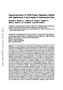
Figure 2: Data from a Poisson Process A key point for any Poisson process is that its expected value is the same as its variance. In a limitless number of independent realizations of a Poisson random variable, the mean of those realizations will be the same as the variance of those realizations. It follows that for real data generated by a Poisson process, the mean should be approximately the same as the variance. This reasoning applies to each λ in the inmate illustration, each representing a different Poisson process.3 We never get to see the equivalent of Figure 1. Figure 1 is a theoretical construct. We get to see realizations of Poisson processes that differ in their values for λ because of age. Figure 2 shows what a set of such realizations might look like and are the data with which an analyst would typically work. When one can make a convincing case that the data to be analyzed were generated by processes consistent with Figures 1 and 2, a Poisson regression can be on sound footing. If the model is on sound footing, the conditional expectations estimated by the fitted values will be the same as the residual variances around those fitted values, save for random error introduced by the Poisson process itself. 3
The Poisson processes are different because they have different values for λ, conditional on age.
5
2.2
Incorrect Functional Forms
Suppose the linear relationship shown in Figure 1 is correct and that a Poisson process applies. However, a different functional form is assumed for the relationships between the conditional expectations of the misconduct counts and age. The truth is linear, but some other functional form such as a quadractic is taken to be true. Over a limitless number of independent realizations of the true Poisson process, the conditional expectations of the assumed Poisson process will differ from the correct ones. The conditional variances around the incorrect conditional expectations will not be the same as the true conditional variances. In fact, the residual variance will too large because it contains the usual random variation and now, systematic error as well. The stage is set for excess variation around the fitted values constructed from real data, which may look a lot like overdispersion. However, the real problem is that the systematic part of the Poisson model has been incorrectly specified.
2.3
Fixed Subject Heterogeneity
It is sometimes possible to argue that the Poisson model fails in a particular manner. Figure 3 is one illustration. There are now three (instead of one) expected values for each value of age, configured so that they are unrelated to age. Similar to Figure 1, Figure 3 represents an unobservable theoretical construct. Figure 4 displays what the resulting realizations might look like if there were three poisson distributions for each age. This is just a particular form of subject heterogeneity, which will suffice for didactic purposes. More extensive discussions of heterogeneity can be found in the influential work Nagin and Land (1993) and in several subsequent papers and books (e.g., Unger et al., 1998, Nagin, 2005). Why might there be three expected values of misconduct by age? One possibility is a failure to consider an important predictor variable. Suppose that in this facility some inmates do not belong to a prison gang, whereas others belong to one of two prison gangs. If such were the case, there could be three different conditional expectations for each age, depending on gang membership, or heterogeneity (as it is often called) in the conditional expectations of misconduct by age. A Poisson model would not properly estimate the misconduct process because it would assume one conditional expectation for each age, when in fact there are three. The fitted values could estimate 6
Fixed Lambda Theory
●
●
●
●
●
●
●
●
●
●
●
●
●
●
●
●
●
●
●
●
●
●
●
●
●
●
●
●
●
●
●
●
●
●
●
●
●
●
●
●
●
●
●
●
●
●
●
●
●
●
●
10
●
5
Number of Incidents
15
●
0
●
20
25
30
35
Years of Age
Figure 3: Fixed Subject Heterogeneity the middle conditional expectation of the three in an unbiased manner, but would fail to capture the full systematic structure in the data. One manifestation would be excess variation around the fitted values compared to the result if the Poisson model were appropriate. Because the three conditional means are a result of an omitted predictor, and because it is conventional to treat all predictors as fixed in the estimation process, the additional heterogeneity can be traced to fixed differences between cases. Figures 3 and 4 allow one to appreciate that even when an omitted predictor is unrelated to an included predictor, there can be excess variability around the fitted values. In practice, omitted variables are likely to be related to included predictors. If gang membership were related to age, the problems with the regression results are more fundamental. Failing to include gang membership in the Poisson regression model leads to biased estimates of the fitted values and the other regression output. For this situation as well, there would likely be excess variation around the fitted values that would look like overdispersion, but the difficulties go deeper. The systematic part of the Poisson model has been misspecified.
7
Realizations for Fixed Lambda
25
●
●
●
●
● ●
15
●
● ●
●
● ●
●
●
●
●
●
●
10
Number of Incidents
20
●
●
●
● ●
●
●
●
● ●
●
● ●
●
●
●
5
● ●
●
●
●
●
●
●
●
●
● ●
0
●
20
25
●
30
●
● ●
35
Years of Age
Figure 4: Data When There Is Fixed Subject Heterogeneity
2.4
Stochastic Subject Heterogeneity
Another explanation for excess variability is that there is random variation in the conditional expectations associated with each age. Every inmate has his/her own conditional expectation that varies independently around an overall expectation for each age. For example, the reported number of misconduct incidents may be measured with error because of mistakes and oversights in what guards are able or willing to record (Poole and Regoli, 1983). If one can assume that the measurement error is essentially “noise” (more details shortly), Figure 5 shows how the pattern of random conditional expectations could appear. The realizations might then look a lot like those in Figure 6. Were a Poisson regression applied to the data, the fitted values could be estimates of the “true” number of misconduct incidents, but there would be excess variation around the fitted values that would seem to meet the conception of overdisperson traditionally discussed in criminological literature (Sampson and Laub, 1997; Paternoster and Brame, 1997). There are no problems with how the systematic part of the Poisson model has been specified. Rather, the difficulties arise from how the stochastic part of the Poisson model has been specified. There is a new source of random variation not accounted for.
8
20
Stochastic Lambda Theory ● ● ● ● ● ●
15
●
●
●
●
● ● ●
● ●
● ●
●
● ● ●
10
●
● ● ● ●
● ● ●
●
●
● ●
● ●
●
● ●
5
Number of Incidents
● ●
●
● ● ●
●
● ●
● ● ●
0
● ●
●
20
25
30
35
Years of Age
Figure 5: Random Subject Heterogeneity
25
Realizations for Stochastic Lambda ●
20
●
●
● ●
●
●
15
●
● ●
●
● ● ●
● ●
●
●
●
●
10
Number of Incidents
●
●
●
● ●
●
●
● ●
●
●
● ●
●
●
●
●
5
● ●
● ● ●
●
●
●
●
0
●
20
25
30
● ●
35
Years of Age
Figure 6: Data When There Is Random Subject Heterogeneity 9
2.5
Dependence Within Counts
Suppose one can argue convincingly that there are no omitted variables altering the conditional expectations in a fixed manner, the functional forms are correct, and there is no random variation in the conditional expectations. Suppose, however, that the acts of misconduct occur in clusters. For example, insubordination, failing to reported for a work assignment, and threatening a guard might all be part of one “acting out” incident. The three acts of misconduct are not independent of each other, as the Poisson model requires. This can lead to a “lumpy” distribution of the counts that is too variable for the Poisson model. In other words, the systematic part of the Poisson model responsible the conditional expectations is correct, but there is a now another kind of error in how the stochastic part is formulated. There is a lack of independence in the events that constitute each count. Then, if a Poisson model is assumed for a particular set of observations, there will be excess variation around the fitted values, which also is consistent with the definition of overdispersion. In principle, there can be underdispersion if the events constituting the counts are negatively related. For example, given a severe shortage of prison beds, a sentencing judge might be reluctant to incarcerate too many convicted felons. If a few convicted felons are sentenced to long prison terms, some subsequent convicted felons, who would ordinarily do time behind bars, could be more likely to receive probation. The issues that underdispersion raises are essentially the same issues that overdispersion raises. In practice, research in criminology seems more concerned about overdispersion, so that is our focus here.
2.6
Some General Lessons
There are at least four reasons why there can be excess variation around the conditional expectations of a Poisson regression model. First, there may be omitted predictors. Second, the functional forms specified may be incorrect. Third, there may be random variation in the conditional expectations. Fourth, they may be dependence between the events that constitute each count. As will be shown more formally below, overdispersion is not just any excess variation in the conditional distributions of count data. Excess variation due to omitted variables, or other errors in the systematic part of a model is 10
not overdispersion. Overdispersion is excess variation when the systematic structure of the model is correct. Overdispersion stems from how the stochastic component of the model is formulated. In criminology, overdispersion has been incorrectly interpreted as any excess variation in the conditional distributions of crime count data. What might criminologists do to address excess variation in conditional distributions of crime count data? When the problem is one or more omitted variables, there is only one solution. The analysis must be undertaken again with formerly omitted variables included. This is especially important if any of the omitted variables are related to included predictors, which is likely in criminological context where there are usually many potential explanatory variables. The same conclusions follow when incorrect functional forms are used. The errors need to be corrected. In short, when there are errors in the systematic part of the Poisson model, there is no fix that will work short of getting the systematic part right. If the systematic part of the model is correct — there are no omitted variables and the functional forms are appropriate — and there is excess variation around the fitted values, stochastic conditional expectations may be the cause. Suppose that the stochastic variation is a result of measurement error in the response that has all of the usual properties of the normal regression disturbance term (Greene, 2003: 84). If these very demanding assumptions can be justified for the application at hand, there should be some useful results from a Poisson regression. In our example, the fitted values can estimate the conditional expectations for each age in an unbiased manner. But the statistical inference from the Poisson regression will be incorrect because the excess variation is not taken into account. A potential solution is to replace the Poisson distribution on which Poisson regression is built with the negative binomial distribution. More will be said about this shortly. When the problem is dependence between the events that go into each count, the consequences and potential solutions are like those for when there are stochastic conditional expectations. Under the Poisson distribution, any statistical inference is suspect. But a potential solution may exist with the negative binomial distribution. Two important issues naturally follow. First, for a real data analysis in which there is evidence of excess variation around the fitting values, can one determine if the problem is an error in the systematic part of the model or the stochastic part of the model (or both)? Second, if the problem lies solely in how the stochastic component is specified, can one determine whether 11
the negative binomial distribution is properly capturing the excess variation around the conditional means? To address these questions we need to get a bit more formal.
3
A More Formal Treatment
It may be useful to start back at the beginning. The Poisson distribution for case i can be written as Prob(Yi = yi |xi ) =
e−λi λyi i , yi !
(1)
where Yi is the random variable representing a count, yi is a particular count value (e.g., 3), λi is the sole parameter representing the expected value of the count, and i = 1, 2, . . . N indexes the N cases. A key premise is that the events constituting each count are independent. If this is not true, the Poisson does not apply. When there is interest in capturing any systematic variation in λi , the value of λi is most commonly placed within a loglinear model ln λi = xT i β,
(2)
where xTi β is the usual linear combination of predictors for case i. It follows that the expected number of events per period for case i (e.g., acts of misT conduct per year a particular inmate) is λi which equals exi β . Equation 2 is sometimes called the mean function. The exponentiation explains why it can be helpful to exponentiate the regression coefficients when Poisson regression output is interpreted. The parameters of equation 2 can be estimated by maximum likelihood, and the usual asymptotic properties follow. A key point is that equations 1 and 2 are theoretical constructs that may or may not apply to a real data set. For example, if there are omitted predictors, equation 2 does not hold. To use equation 2 nevertheless is to risk serious problems. Likewise, it can be risky to proceed if the events constituting each count are not independent.
3.1
Introducing Random Variation in λi
As discussed earlier, one can introduce random variation into λi . Noisy measurement of the count may be the motivation. Following Greene (2003: 12
744-745), one can write ln µi = xT i β + εi ,
(3)
where εi is rather like a conventional disturbance in normal regression. Each εi has an expected value of zero and the same variance, and each is generated independently of one another. Because of εi , µi is a noisy version of λi . Even for a single case, the value of λi can change over realizations of the data, and cases with the same set of predictor values will generally not have the same value of λ. (Look again at Figure 5.) One can think of the count now as a “doubly stochastic Poisson” (Cox, 1955) because in addition to the uncertainty built into the Poisson formulation, there is second source of uncertainty from εi . It is important to appreciate that in this formulation, the xTi β is correct in the usual sense.4 There are no omitted variables, and the functional forms are the right ones. In other words, the systematic part of the model is sound. To move toward a procedure to estimate the regression coefficients, still more needs to be assumed about the properties of εi . The Poisson formulation can then be altered so that e−λi µi (λi µi )yi , (4) f (yi |xi , µi ) = yi ! which means that conditional upon xi and µi , the distribution of the yi remains Poisson. But, that begs the question. One wants to characterize the distribution of yi conditional only on xi , because it is xi that is observable. This requires first that the density of ui (and implicitly εi ) be specified. “For mathematical convenience, the gamma distribution is usually assumed for µi = eεi .” (Greene, 2003: 745). After normalizing the gamma distribution to have an expected value of 1.0,5 one arrives at θθ −θµi θ−1 e µi , (5) Γ(θ) where Γ denotes the gamma distribution, and θ is a parameter to be specified a priori or estimated. Integrating over ui , the density for yi , conditional only on the predictors, is g(ui ) =
f (yi |xi ) = 4 5
Γ(θ + yi ) yi r (1 − ri )θ , Γ(yi + 1)Γ(θ) i
This follows from the assumptions about εi . Without normalization, the model’s constant would not be identified.
13
(6)
where
λi . (7) λi + θ This gets us to the negative binomial distribution. The expected value for each case is λi , which corresponds to the Poisson. This is a very important relationship because it implies that the expected value for the mean function is the same whether the Poisson distribution is used or the negative binomial distribution is used. On the average they are trying to estimate the same thing. It might not be surprising to find, therefore, that in practice the estimated regression coefficients from the two procedures are much alike. So, if there are problems with the mean function when the Poisson distribution is used, those problems are likely to remain when the negative binomial distribution is used. The variance of the conditional mean λi is not λi , but λi [1 + (1/θ)λi ]. For θ > 0, the variance is inflated, presumably to address overdispersion. The smaller the value of θ > 0, the greater the overdispersion. But whatever the value of θ, each λi is multiplied by the same factor. This is a very special flavor of overdispersion in which each conditional variance is inflated by exactly the same factor. It would imply, using the prison example, that the reporting practices of guards would introduce precisely the same proportional increase in noise on the average whether a large number or small number of misconduct incidents had actually occurred. Such an assertion would need to rest on sound theory or credible past research.6 With the density in hand, the values of β can be estimated by maximum likelihood, and a one-tailed test that θ = 0 can be used to determine the strength of the evidence for overdispersion. In short, given that the systematic part of the model is correct, the negative binomial can in principle address overdisperson of a particular kind. ri =
3.2
Some Statistical Implications
The formal derivation of how overdispersion can be addressed by the negative binomial distribution underscores several important statistical points. To begin, it is critical to distinguish between the possible reasons why the variance around the fitted values seems too large. The remedies, such as 6
If θ = 0, one is back to the Poisson distribution. One can view the negative binomial distribution as a particular generalization of the Poisson. If θ < 0, there is underdispersion.
14
they are, can be very different. When the systematic part of the Poisson regression is incorrect, there can be excess variation around the fitted values. As a definitional and formal matter, this is not overdispersion. The solution is to fix how the systematic part of the model is specified. Overdispersion assumes that the systematic part of the Poisson regression is correct. The problems stem from how the stochastic part of the model is formulated. The solution is to reformulate the stochastic part of the model. Choosing an alternative distribution to the Poisson is often recommended. It is very unlikely that one can empirically distinguish between excess variation around the fitted values because of mispecification of the systematic part of the model and excess variation around the fitted values because of mispecification of the stochastic part of the model. Typically, the case needs to be made on theoretical grounds or from the results of earlier studies. There rarely will be a direct link between how one understands the processes by which the overdispersion is generated and the use of the negative binomial distribution. It is a marriage of convenience. There are other distributions that can be used, which can lead to different empirical results, and the other distributions will generally be just as arbitrary (Cameron and Trivedi, 1998: chapter 4). Also, there is usually no way empirically to choose between two sets of arbitrary results. Moreover, to find that two or more competing models lead to similar substantive conclusions does not mean that those conclusions are correct. All of the models used in the analysis may be wrong. We illustrate this point shortly. Finally and perhaps most important, Poisson regression and negative binomial regression are responding to the same expected mean function. One might not anticipate much difference in the regression coefficients estimated. So, if the estimated regression coefficients from a Poisson regression are biased and inconsistent, the estimated regression coefficients from a negative binomial regression will be as well. What the negative binomial brings to the table is the hope of getting the variance of λi about right for a model that is otherwise properly specified. With a better fix in the variance of λi , more reasonable standard errors can follow.
3.3
Some Implications for Practice
There is a natural ordering to how one should proceed in practice. First, if at all possible, one should build a Poisson regression model for which there are no apparent omitted variables and for which the correct functional forms 15
are used. Both will depend heavily on sound theoretical arguments and the results of past criminological research. Simply assuming that all is well will not do. Second, if a strong case cannot be made that the systematic part of the model is essentially correct, the modeling exercise may be over. There is a good fallback position, however. One can undertake a descriptive data analysis. What exactly this entails is discussed elsewhere (Berk, 2003) and is beyond the scope of this paper. Third, if a strong case can be made that the systematic part of the model is essentially correct, and if there then is overdispersion, the regression estimates may still be sufficiently sound. But statistical inference is probably not. Hypothesis tests and confidence intervals will not perform as they are intended. If statistical inference is not an important part of the analysis, there may be no need to search for a remedy. Fourth, if a remedy is needed, using the negative binomial distribution is one option. But one must be clear that there are other options, and none are likely follow from understandings about what is causing the overdispersion. Moreover, there is no way to determine empirically if the “patch” is leading to correct statistical inference or not. Finally, should one really have errors in the systematic part of the model and nevertheless proceed as if there is overdispersion, the true problems are being papered over. The result can be regression output with little substantive meaning. Note that just because the p-values for various statistical tests are smaller does not mean that one is better off, as we show below.
4
An Illustration
The way in which the negative binomial can obscure model specification errors is easy to illustrate with a simple simulation. One can construct a data set for which the values of the population parameters are specified a priori. Because the true parameter values are known, it is then straightforward to consider what happens when the wrong model is used and how effective a proposed remedy really is. In short, the goal is to use simulation techniques to compare various estimators. This is a common practice in statistics (Ripley, 2007). If real data were used instead, there is no easily ascertained truth to use as a benchmark. There is, therefore, no compelling way to document 16
the consequences of modeling errors or whether a proposed remedy really provides the requisite fix; one cannot determine if a fix works unless the correct answer is known. Fortunately, there is no penalty in this case for relying on a simulation because the points to be made carry over directly when real data are analyzed. Using the programming language R, 500 realizations from a particular conditional Poisson process was constructed in the following manner. 1. Values for three predictors with 500 observations each were sampled from a specified multivariate normal distribution. The use of the normal compared to some other distribution is immaterial because in regression analysis one usually conditions on the predictors. A covariance matrix was used that generated random variables with moderate correlations of around .40. Correlations of around this size are often found criminology research that relies on negative binomial regression (Osgood and Chambers, 2000). The conclusions to follow would not be materially different had substantially smaller or substantially larger correlations been used. The result was a 500 by 3 design matrix with columns x1 , x2 , x3 . 2. As the generalized linear model requires, a linear combination of the three predictors was constructed. Specifically, the linear combination was −2 + 1(x1 ) + 2(x2 ) − 1.5(x3 ). The coefficients represent the population parameters. The conclusions to follow do not depend importantly on the particular coefficient values used. 3. The linear combination of predictors was exponentiated, as the canonical link for Poisson regression requires. 4. The exponentiated values were used as conditional means for 500 draws from a Poisson distribution. The Poisson realizations became the values for the response variable. Table 1 shows the results when the simulation data were analyzed. Under the column labeled “Truth” are values of population parameters as defined by the simulation. These are the values one is trying to estimate. The column labeled “Correct Model” shows the estimates produced when the correct Poisson model is applied to the constructed data. In contrast to most empirical work with real data, we know exactly what the correct model 17
must be. Therefore, all of the parameter estimates are necessarily within random sampling error of the truth. In this case, if the population values are used as the null hypothesis for each coefficient, one could not reject the null hypothesis at the .05 level. The residual deviance is 511.6, approximately equal to the residual degrees are freedom, which is one indication that the model is performing as it should. In short, all looks well. Predictor
Truth
Const. x1 x2 x3 Res. Dev.
-2 1 2 -1.5 ——–
True Model -1.81 (.55) 1.09 (.23) 1.70 (.18) -1.37 (.17) 511.6
Drop x2 -0.13 (.52) 2.04 (.21) ——– -1.22 (.17) 603.3
Drop x2 , x3 -1.57 (.48) 1.32 (.17) ——– ——– 653.9
NB Drop x2 -0.12 (.57) 2.04 (.23) ——-1.22 (.19) 501.0
NB Drop x2 , x3 -1.56 (.55) 1.32 (.21) ——– ——– 503.2
Table 1: Simulation Results: Regression Coefficients, Standard Errors and Residual Deviance The column labeled “Drop x2 ” shows the results when x2 is removed from the correct model; x2 becomes an omitted variable. The constant is now approximately zero, the regression coefficient for x1 is nearly doubled, and the regression coefficient for x3 is about the same. If doubling the regression coefficient for x1 does not seem sufficiently troubling, note that when exponentiated, the count multiplier increases from 2.97 to 7.69. Standard errors are reported although because of the omitted variable, they are suspect. The two sets of Poisson regression results are clearly different and as a formal matter, the estimates for the second model are biased and inconsistent. It would have been easy to construct a simulation in which changes resulting from an omitted variable would have been far more dramatic, but for reasons that will soon be apparent, we wanted the misspecification impacts to be modest. At the bottom of Table 1, one can find, where appropriate, the residuals deviances. When x1 is disarded, the residual deviance increases from 511.6 to 603.3. This is clear evidence of overdispersion; compared residual deviance for the correct model, the new residual deviance is greater by nearly 100 (about a 20% increase). One can easily flesh this out by looking at the conditional variances for different conditional means. For example, under 18
the correct model, the conditional variance is 4.9 when the conditional mean between 4.5 and 5.5.7 This is just what one would expect. When the misspecified model is used instead, the conditional variance is over 6.0. Similarly, under the correct model, the conditional variance is 9.4 when the conditional mean between 8.5 and 9.5. When the misspecified model is used instead, the conditional variance is over 11. In short, the conditional variance is about the same as the conditional mean for the correct model, but the conditional variance is somewhat larger than the conditional mean under the incorrect model. There looks to be overdispersion, which follows directly when the required predictor x2 is discarded. In the column labeled “Drop x2 , x3 ” are the results when x2 , and x3 are removed. The two missing predictors as implicitly assumed to have regression coefficients of 0.0, which is clearly incorrect. The empirical results are biased and inconsistent, and the residual variance is even larger. The apparent overdispersion is worse. The last two columns show for the two misspecified models the results when the Poisson distribution is replaced by the negative binomial distribution. For both models, estimates of θ from equations 5 - 7 are positive. When the negative binomial distribution is applied, there is additional statistical evidence for overdispersion. In the face of this apparent overdispersion, the critical question is whether using the negative binomial distribution leads to estimated regression coefficients that are within sampling error of true parameter values. That is, are the estimated coefficients much like those produced by the correct model or are they much like those produced by the two incorrect models? If the applying the negative binomial distribution is really doing what some claim it should, the former should found. As anticipated by the formal material presented earlier, the estimated regression coefficients for the models that are known to be incorrect are almost exactly reproduced. For example, when the Poisson model is applied after x2 is removed, the estimated regression coefficient is 2.04. When the negative binomial model is applied after x2 is removed, the estimated regression coefficient is 2.04. The true value is 1.0, and the value obtained from the correct model is 1.09. In fact, all such comparisons, including the regression constants, lead to differences in only in the second decimal place. Increas7
In order to have sufficient observations to get a good reading on the conditional variance, ranges of conditional means are used.
19
ing the number of observations in the simulation to as high as 50,000 does not materially change these comparisons. The results do not depend on the sample size of 500, which is large but hardly “asymptotic.” Finally, there is the matter of statistical tests. In this simulation, and others much like it that we examined, the standard errors for both the misspecified Poisson regression and the misspecified negative binomial regression were about the same, and also about the same as the standard errors for the correctly specified Poisson regression. However, the p-values for the misspecified models are widely off target because of the bias in the regression coefficients from the misspecified models. For example, the correct p-value associated with the regression coefficient for x1 reflects the disparity between 0.0 (i.e. the null hypothesis) and 1.09. But for the misspecified models, the p-values reflect the disparity between 0.0 and 2.04. So, even though the standard errors do not change much, the z-values are about twice as large, and the p-values are reduced several orders of magnitude. Smaller p-values are not by themselves evidence for an improved model. In summary, the omitted variable bias we introduced was relatively modest by intent and of a magnitude consistent with much common practice. One might think, therefore, that a recommended remedial procedure would get the job done. We were not asking for anything remarkable. Yet, the misspecified Poisson regression model and the negative binomial model produce regression coefficients that are virtually identical. There is no evidence that using the negative binomial distribution instead of the Poisson distribution helps when the systematic part of a regression model is misspecified.
5
Summary and Conclusions
Count data are common in criminal justice research. Poisson regression can be a useful in the analysis of such data. But Poisson regression is subject to all of the usual concerns about regression (Berk, 2003). Some have claimed when Poisson regression fails because of overdispersion, turning to the negative binomial distribution can provide a remedy (Osgood, 2000). If apparent overdispersion results from specification errors in the systematic part of the Poisson regression model, resorting to the negative binomial distribution does not help. It can make things worse by giving a false sense of security when the fundamental errors in the model remain. If there is true overdispersion as a result solely of specification errors in that stochastic part 20
of the Poisson regression model, trying to correct those errors can be useful. However, arriving at the proper fix is very difficult. There is no necessary connection between the the reasons for the mispecification and one or more alternatives to the conventional Poisson distribution. One risks an arbitrary correction leading to arbitrary results. In practice, it is likely that excess variation around fitted values results from specification errors in the systematic part of the Poisson regression model: omitted variables and incorrect functional forms (Box, 1976; Freedman, 1987; de Leeuw, 1994; Manski, 1990; Heckman, 1999; Berk, 2003). It makes sense, therefore, to concentrate one’s efforts on getting the systematic structure right. Only after a convincing case has been made that the systematic structure is effectively correct should one turn to concerns about the structure of the stochastic component.
21
References Berk, R.A. (2003) Regression Analysis: A Constructive Critique. Newbury Park, CA.: Sage Publications. Box, G.E.P. (1976) “Science and Statistics.” Journal of the American Statistical Association 71: 791-799. Bottcher, J., and M.E. Ezzell (2005) “Examining the Effectiveness of Boot Camps: A Randomized Experiment with Long-Term Follow Up,” Journal of Research in Crime and Delinquency 42: 309-332. Braga, A. (2003) “Serious Youth Gun Offenders and the Epidemic of Youth Violence in Boston,” Journal of Quantitative Criminology 19: 33-54. Cameron, A.C. and P.K. Trivedi (1998) Regression Analysis of Count Data. Cambridge: Cambridge University Press. Cox, D.R. (1955) “Some Statistical Models Related with A Series of Events.” Journal of the Royal Statistical Society B 17: 406-424. de Leeuw, J. (1994) “Statistics and the Sciences,” in Trends and Perspectives in Empirical Social Science, I. Borg and P.P. Mohler (eds.), New York: Walter de Gruyter. Duwe, G., T. Kovandzic, and C. Moody (2002) “The Impact of Right-toCarry Concealed Firearm Laws on Mass Public Shootings,” Homicide Studies 6: 271-296. Freedman, D.A. (1987) “As others See Us: A Case Study in Path Analysis.” (with discussion). Journal of Educational Statistics12: 101-223. Freedman, D.A. (2005) Statistical Models: Theory and Practice. CAmbridge: Cambridge University Press. Greene, W.H. (2003) Econometric Analysis, fifth edition. New York: Prentice Hall. Heckman, J. (1999) “Causal Parameters and Policy Analysis in Economics: A Twentieth Century Retrospective,” The Quarterly Journal of Economics, February: 45-97. 22
Lattimore, P. K., J. M. MacDonald, A. R. Piquero, R. L. Linster, and C. A. Visher (2004) “Studying Frequency of Arrest Among Paroled Youthful Offenders,” Journal of Research in Crime and Delinquency 41: 37-57. Manski, C.F. (1990) “Nonparametric Bounds on Treatment Effects.” American Economic Review Papers and Proceedings 80: 319-323. McCullagh, P., and J.A. Nelder (1989) Generalized Linear Models, second edition. New York: Chapman and Hall. Morgan, S.L. and C.Winship (2007) Counterfactuals and Causal Inference: Methods and Principle for Social Research, Cambridge: Cambridge University Press. Ripley, B.D. (2006) Stochastic Simulation. New York, John Wiley and Sons. Parker, K. (2004) “Industrial Shift, Polarized Labor Markets and Urban Violence: Modeling the Dynamics between the Economic Transformation and Disaggregated Homicide,” Criminology 42: 619-645. Paternoster, R., and R. Brame (1997) “Multiple Routes to Delinquency? A Test of Developmental and General Theories of Crime,” Criminology 35: 45-84. Paternoster, R., R. Brame, R. Bachman, and L. Sherman (1997) “Do Fair Procedures Matter? The Effect of Procedural Justice on Spouse Assault,” Law and Society Review 31: 163-204. Nagin, D.S., and K.C. Land (1993) “Age, Criminal Careers, and Population Heterogeneity: Specification and Estimation of a Nonparametric, Mixed Poisson Model,” Criminology 31: 501-523. Nagin, D.S. (2005) Group-Based Modeling of Development. Cambridge: Harvard University Press. Piquero, A. R., J. M. MacDonald, and K. F. Parker (2002) “Race, Local Life Circumstances, and Criminal Activity,” Social Science Quarterly 83: 254-270. Poole, E.E. and R.M. Regoli (1983) “Violence in Juvenile Institutions,” Criminology 21: 213-232. 23
Osgood, W. (2000) “Poisson-based Regression Analysis of Aggregate Crime Rates.” Journal of Quantitative Criminology 16: 21-43. Osgood, D. W., and Chambers, J. M. (2000). ”Social disorganization outside the metropolis: An analysis of rural youth violence.” Criminology 38: 81115. Sampson, R.J., and J. H. Laub (1997) “Socioeconomic Achievement in the Life Course of Disadvantaged Men: Military Service as a Turning Point, Circa 1940-1965,” American Sociological Review 61: 347-367. Stucky, T.D. (2003) “Local Politics and Violence Crime in U.S. Cities,” Criminology 41: 1101-1135.
24