Black-Box Algorithms for Sampling from Continuous ... - IEEE Xplore

Proceedings of the 2006 Winter Simulation Conference L. F. Perrone, F. P. Wieland, J. Liu, B. G. Lawson, D. M. Nicol, and R. M. Fujimoto, eds.

BLACK-BOX ALGORITHMS FOR SAMPLING FROM CONTINUOUS DISTRIBUTIONS Josef Leydold Wolfgang H¨ormann Department of Statistics and Mathematics Vienna University of Economics and Business Administration Augasse 2-6, 1090 Vienna, AUSTRIA

•

ABSTRACT For generating non-uniform random variates, black-box algorithms are powerful tools that allow drawing samples from large classes of distributions. We give an overview of the design principles of such methods and show that they have advantages compared to specialized algorithms even for standard distributions, e.g., the marginal generation times are fast and depend mainly on the chosen method and not on the distribution. Moreover these methods are suitable for specialized tasks like sampling from truncated distributions and variance reduction techniques. We also present a library called UNU.RAN that provides an interface to a portable implementation of such methods. 1

•

INTRODUCTION

From a theoretical point of view non-uniform random variate generation can be seen as a procedure where a given sequence of i.i.d. uniformly distributed random numbers is transformed into a sequence of random variates that follow the target distribution. (There is hardly any paper that proposes a nonuniform random variate generator without the help of a uniform random number generator.) Many algorithms that are especially tailored for particular distributions have been developed for this task, see Devroye (1986). Design goals for these algorithms are speed and little memory consumption, sometimes particular simulation problems. From a practitioner’s point of view random variate generation happens somewhere inside a routine provided by some programming library. For her it is only important that the library of choice (i) provides such a routine for her particular distribution and (ii) the generated point set is of “good quality”, i.e., the results of her stochastic simulation is reliable. These different points of view raise some problems when running a stochastic simulation:

1-4244-0501-7/06/$20.00 ©2006 IEEE

•

When there is no routine for the required distribution, one needs to look for a different library, or has to implement (and test!) some algorithm found in literature by herself, or even worse has to design such an algorithm. However, the latter requires great expertise. Sometimes generic generation routines are provided. However these often use inaccurate brute force methods and should be used with extreme care. The theory of generation methods is based on the assumption that we have truly random numbers and that the calculations are conducted in the field of real numbers R. Neither is true in real world simulations as we only have pseudo-random number with restricted resolution and all computers use floating point numbers, see Overton (2001) for an overview of handling such numbers. Thus extensive tests with each of these generators would be necessary to guarantee reliability in all simulation studies. The arguments of sampling routines depend on the particular distributions. Thus running a simulation with (slightly) different input distributions can be difficult to implement. There also exist programming environments where the underlying uniform random number generator is set by a global variable. Hence running streams of (common or independent) random numbers is difficult to implement.

Black-box (also called automatic or universal) algorithms are an important recent development in random variate generation. Such algorithms are designed to work with large classes of distributions. The advantages of such an approach compared to specialized generating methods are obvious:

129

Leydold and H¨ormann • •

•

• •

Only one piece of code, implemented and exhaustively tested once, is required. Automatic methods can be applied by users with little (or even no) experience in random variate generation. They only have to provide some information about the target distribution, typically its probability density function (PDF) together with some extra information like its mode. The quality and structural properties of point sets generated by such algorithms do not depend on the particular distribution but only on the chosen method. Thus it is possible to choose a method that is best suited for the application. The performance of these algorithms often does not depend on the target distribution. These methods work equally well for non-standard distributions where no special generation methods exist. One only has to check whether the assumptions for the black-box algorithm are satisfied.

1

U

X Figure 1: Inversion Method • •

Consequently, it can be used for variance reduction techniques as well as in the framework of quasi-Monte Carlo simulation where highly uniformly distributed point sets are used. It is also easy to sample from truncated distributions. Moreover, the quality of the generated random variates only depends on the underlying uniform PRNG, not on the distribution. Hence it is the method of choice in simulation literature, see, e.g., Bratley, Fox, and Schrage (1983). Unfortunately, the inversion method requires the evaluation of the inverse of the CDF which is rarely available except for special cases like the exponential distribution. Thus numerical methods to invert the CDF have to be used, most prominently Newton’s method and regula falsi. However, such methods are (very) slow and it is only possible to improve them using large tables. Nevertheless, such methods are sometimes used as brute force implementation of generic random variate generators. A fast alternative to such slow methods is to approximate the inverse CDF by a function that is faster to evaluate. Cubic Hermite interpolation is very suitable for this task. To apply this method the CDF and the PDF are evaluated at some construction points ci and for each subinterval [F −1 (ci ), F −1 (ci+1 )] the inverse CDF is interpolated by a polynomial of degree three which has the same values and derivatives at the construction points. An advantage of Hermite interpolation is that it can be improved by splitting single subintervals (i.e., by adding further construction points) without the necessity to recompute the entire interpolation (as for splines). The construction points can be searched automatically by bisectioning subintervals such that the maximal interpolation error is as small as desired and monotonicity of the approximate inverse CDF is guaranteed. The resulting algorithm is very fast and can be used whenever the CDF is available or can be computed by a numerical integration routine. The costs for the latter case are less important as only a few points (typically less

However, it should not be concealed that there are also some drawbacks: Black-box algorithms require a setup step where all constants that are necessary to run the sampling routine are computed, which requires some time and slightly more memory than specialized algorithms. Anyhow, there is a trade off between setup time and marginal generation time which can be controlled by the user. When implemented in a programming library one also needs an application programming interface (API) that allows to pass all required data for the algorithm. Nevertheless, we think that in a modern computing environment the advantages by far exceed the disadvantages even for standard distributions. In this short survey we summarize the main principles of automatic methods for random variate generation and show how such algorithms are implemented in a library called UNU.RAN (Universal Non-Uniform RAndom Variate generators) using an object oriented programming paradigm, see Leydold et al. (2005). For a detailed discussion of modern black-box algorithms we refer the interested reader to the monograph by H¨ormann, Leydold, and Derflinger (2004). 2

It transforms one uniform random number into one non-uniform random number. It preserves the structural properties of the underlying uniform pseudo-random number generator (PRNG).

INVERSION METHOD

The inversion method (see Figure 1) is based on the following observation: Let F(x) be a cumulative distribution function (CDF) and and U a uniform U(0, 1) random number. Then X = F −1 (U) = inf {x : F(x) ≥ U} is a random variate with CDF F. The inversion method is the most general method for generating non-uniform random variates. It has several advantages:

130

Leydold and H¨ormann than 1000) are required. Notice that this method does not evaluate the inverse CDF for a given point directly. (For details see H¨ormann and Leydold 2003). 3

rejection constant. It is important to note that for applying the rejection method f can be any (unknown) multiple of a PDF. Then α might not be known but can be estimated by ρ when we choose hat and squeeze accordingly. For the design of black-box algorithms based on the rejection method we have to construct hat and squeeze automatically. For the design of fast and simple algorithms we have to take care about the following construction principles:

REJECTION METHOD

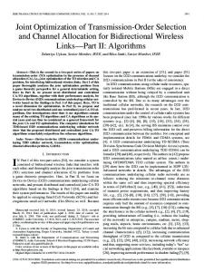
Numerical methods for the inversion method are often either very slow or not exact, i.e., they produce random numbers which follow only approximately the target distribution. When speed and sampling from the exact distribution is crucial the rejection method (see Figure 2) is a suitable alternative. It is based on the following theorem: If a random vector (X,U) is uniformly distributed on

• •

G = {(x, y) : 0 < y ≤ γ f (x)} •

then X has PDF f for every constant γ > 0. Vice versa, for a uniform random number U and a random variate X having PDF f , (X,U γ f (X)) is uniformly distributed on G. Utilizing this theorem we need a majorizing function h(x) (also called hat function) for the PDF f (x), where h is the multiple of some PDF g(x), i.e., f (x) ≤ h(x) = α g(x) for all x. Then generate a random variate X with PDF proportional to h and a (0, 1) uniform random number U. If U h(X) ≤ f (X), return X, otherwise reject X and try again. Simple lower bounds s(x) ≤ f (x), called squeezes, can be used to reduce the number of (expensive) evaluations of f .

•

The hat and squeeze must be easy to compute. It must be possible to sample from the hat distribution easily by inversion. This is necessary as we want to save most of the good properties of the inversion method for the black-box rejection algorithm. For example, it is then easy to sample from truncated distributions. It must be possible to obtain a ratio ρ close to 1. For values near one we hardly have to evaluate the PDF and thus the marginal generation time is almost independent of the target distribution. Moreover, it is “close” to the inversion method. There is a trade-off between setup time (and memory consumption) and marginal generation times which depends on the ratio ρ . Thus it can be controlled by the user.

3.1 Ahrens Method The simplest method for constructing hat and squeeze is to use piecewise constant hat and squeeze functions. It is unbeatable simple in the case of monotone and bounded densities with bounded domains. It can be extended to arbitrary densities as long as the extremal points are known. Ahrens (1995) describes an algorithm (see Figure 3) based on this idea.

1/2

π Figure 2: Rejection Method: PDF f (x) = sin(x)/2 for x ∈ [0, π ], Constant Hat h(x) and Triangular Squeeze s(x)   The constant α = R h(x) dx/ R f (x) dx is called the rejection constant and gives the expected number of iterations to get one random variate. In practice the ratio ρ between the respective areas below hat and below squeeze is more useful  h(x) dx area below hat . = ρ=  area below squeeze s(x) dx

Figure 3: Ahrens Method The main steps of this algorithm for a given density f with domain [a, b] are:

The ratio ρ gives the expected number of evaluations of f to get one random variate and is an upper bound for the

131

Leydold and H¨ormann SETUP: 1.

2.

and Swartz (1998) have shown that this technique is even suitable for arbitrary densities provided that the inflection points of the transformed density are known. It should be noted here that the tangent on the transformed density can be replaced by secants through two points that are close together, shifted away from the mode by the distance of these two points. Thus no derivatives are required. Algorithms based on TDR work similar to the Ahrens method: Choose construction points ci ; compute subintervals where the tangent at ci forms the hat function; compute the volumes below the hat for each subinterval. The generator part works similar as well but rejection from a constant hat is replaced by general rejection. There exist many variants of this basic algorithm. For a complete reference we refer to Chapter 4 of H¨ormann et al. (2004). It is obvious that the transformation T must have the property that the area below the hat is finite, and that generating a random variable with density proportional to the hat function by inversion must be easy (and fast). Thus we have to choose the transformations T carefully. H¨ormann (1995) suggests the family Tc of transformations, where

Select constructions points a = c0 , c1 , c2 , . . . , cn = b and construct hat hi and squeeze si for each subinterval [ci−1 , ci ]. Compute areas below hat in each subinterval, Hi = hi (ci − ci−1 ).

GENERATOR: 3. 4. 5. 6. 7.

Generate I with probability vector proportional to (H1 , . . . , Hn ). Generate X ∼ hI (by inversion) and U ∼ U(0, 1). If U h(X) ≤ s(X), return X. If U h(X) ≤ f (X), return X. Otherwise goto 3 and try again.

Sampling step 3 can be executed in constant time, i.e., independent of the number n of subintervals, by means of indexed search (Chen and Asau 1974). Notice that the uniform random number that is necessary for drawing the discrete random variable I can be recycled (H¨ormann et al. 2004, § 2.3.2) for step 4. Thus sampling X is done by means of the inversion method. The marginal generation times of this algorithm are extremely fast and the ratio ρ can be made as close to 1 as desired. It can be even improved since we have a region of “immediate acceptance” below the squeeze, where no uniform random number U is required. That is, we have a mixture of distributions with PDF proportional to squeeze s(x) and h(x) − s(x), respectively. The drawback of this simple algorithm is that we have to cut off tails in case of unbounded domains and of regions near a pole in case of unbounded densities. This is no problem as long as these regions are not of “computational relevance”, i.e., when their probability is negligible. Moreover, the convergence of ρ towards 1 is rather slow.

T0 (x) = log(x)

and

Tc (x) = sign(c) xc .

(1)

(sign(c) makes Tc increasing for all c.) For densities with unbounded domain we must have c ∈ (−1, 0]. For the choice of c it is important to note that the area below the hat increases when c decreases. Moreover we find that if f is Tc -concave, then f is Tc -concave for every c ≤ c (H¨ormann 1995). Because of computational reasons, the choice of c = −1/2 (if possible) is suggested. This includes all logconcave distributions. Table 1 gives examples of T−1/2 concave distributions. 3.3 Construction Points

3.2 Transformed Density Rejection

The proper choice of construction points is crucial for both algorithms, Ahrens method and TDR. We want to have a small ratio ρ with a small number of construction points. There are several options:

Transformed density rejection (TDR) is a very flexible method. It has been introduced under a different name by Gilks and Wild (1992), and was generalized by H¨ormann (1995). It is based on the idea that the given density is transformed by a strictly monotonically increasing transformation T : (0, ∞) → R such that T ( f (x)) is concave. We then say f is T -concave; log-concave densities are an example with T (x) = log(x). By the concavity of T ( f (x)) it is easy to construct a majorizing function for the transformed density as the minimum of several tangents. Transforming this function back into the original scale we get a hat function h(x) for the density f . By using secants between the touching points of the tangents of the transformed density we analogously can construct squeezes. Figure 4 illustrates the situation for the standard normal distribution and T (x) = log(x). Evans

•

•

132

Simple heuristics: equal-area rule (construct subintervals such that all have the same area Hi below the hat) and equidistributed points (use ci = tan(−π /2 + i π /(n + 1)), i = 1, . . . , n). These work astonishingly well for “well-behaved” densities. Adaptive rejection sampling (ARS). Start with a hat function with a few construction points and run the generator. Whenever we have to evaluate f at X use this point as new construction point and thus decrease ρ in the corresponding subinterval.

Leydold and H¨ormann

Figure 4: Hat Function and Squeeze with Three Points of Contact for the Normal Distribution and Logarithm as Transformation: Transformed Scale (Left) and Original Scale (Right)

Table 1: T−1/2 -Concave Densities (Normalization Constants Omitted)

•

•

Distribution

Density

Normal Log-normal Exponential Gamma Beta Weibull Perks Gen. inv. Gaussian Student’s t Pearson VI Cauchy Planck Burr Snedecor’s F

e−x /2 1/x exp(− ln(x − μ )2 /(2σ 2 )) λ e−λ x xa−1 e−b x xa−1 (1 − x)b−1 xa−1 exp(−xa ) 1/(ex + e−x + a) xa−1 exp(−bx − b∗ /x) (1 + (x2 /a))−(a+1)/2 xa−1 /(1 + x)a+b 1/(1 + x2 ) xa /(ex − 1) xa−1 /(1 + xa )b xm/2−1 /(1 + m/n x)(m+n)/2

2

De-randomized adaptive rejection sampling (DARS). Similar to ARS. For all subintervals where the area between hat and squeeze is larger than a threshold value a new construction point is inserted. Optimal construction points. There exist sophisticated algorithms for finding such points at adequate time, see Section 4.4 in (H¨ormann et al. 2004).

Support

T−1/2 -concave for

R [0, ∞) [0, ∞) [0, ∞) [0, 1] [0, ∞) R [0, ∞) R R R [0, ∞) [0, ∞) [0, ∞)

√ σ≤ 2 λ >0 a ≥ 1, b > 0 a, b ≥ 1 a≥1 a ≥ −2 a ≥ 1, b, b∗ > 0 a≥1 a, b ≥ 1 a≥1 a ≥ 1, b ≥ 2 m, n ≥ 2

same uniform random numbers for both streams, for negative correlation (antithetic variates) we take U for the first stream and 1 −U for the second one. However, correlation induction also works for the rejection method. Following Schmeiser and Kachitvichyanukul (1990) we have the following recipe: Use two independent streams of uniform random numbers. When drawing one random variate use stream 1 for the first acceptance/rejection step. If the point is rejected switch to the auxiliary stream 2 until a point is accepted. Start the next iteration with stream 1 again. Thus streams of non-uniform random variates keep synchronized and correlation is only affected whenever rejection happens in one of the streams. Again a value close to 1 for the ratio ρ is important which is possible for automatic algorithms.

3.4 Correlation Induction Common random numbers and antithetic variates are two of the best known variance reduction techniques for simulation experiments. Both methods require the generation of correlated random variates. Using the inversion method it is no problem to induce the strongest possible positive or negative correlation when generating two random variate streams (even with different distributions). For positive correlation (common random numbers) we simply use the

133

Leydold and H¨ormann 3.5 Multivariate Distributions

ter object is created that holds a marker for the chosen algorithm together with these parameters. These default values can then be changed on demand. We can select TDR with parameter c = 0 (T (x) = log(x)) by

One important advantage of the rejection method is that it can also be used to generate random vectors, in contrast to the inversion method. Even the principle of TDR can be generalized easily to multivariate log-concave or T -concave distributions as we can use tangential hyperplanes of the transformed density to construct hat-functions. The implementation of the details is of course much more complicated than in the univariate setting. Nevertheless it is possible to construct TDR-based black-box algorithms for log-concave densities that work well up to dimension five and acceptable up to dimension ten. Figure 5 illustrates the situation on a simple example. For details see Section 11.3 in (H¨ormann et al. 2004) and the references given there. It is obvious that also the principle of the Ahrens method can be easily generalized to higher dimensions. But due to the bad fit of the constant hat function the necessary number of intervals explodes so fast that its use is limited mainly to two and three-dimensional distributions. 4

par = unur_tdr_new(distr); unur_tdr_set_c(par,0.);

3.

4.

Select a source of randomness. The library can work with any source of uniform random numbers. The source can be set for each instance of a parameter object (or changed for each instance of a generator object). Thus is is easy to switch the underlying URNG “on the fly”. An excellent source of multiple random streams which is well suited to work with UNU.RAN is the RngStreams package developed by L’Ecuyer et al. (2002). When no generator is set explicitly, a global generator is used. Initialize the generator. This executes the setup of the algorithm and computes all necessary tables.

UNU.RAN gen = unur_init(par);

We have implemented most of the important black-box algorithms described in the monograph H¨ormann et al. (2004) in a library called UNU.RAN which can be downloaded from our website (Leydold et al. 2005). It has been coded in ANSI C using an object oriented programming paradigm. The design of an API for black-box algorithms for random variate generation requires an approach that is different from the “traditional” style. We use four different types of objects: a distribution object holds the necessary data for the required distribution like pointers to the PDF or the mode; a parameter object for the chosen methods and its parameter, a URNG object that is used as source of uniform random numbers, and a generator object that is used to generate random variates. Thus we have the following steps: 1.

2.

5.

Run the generator. It can be used to draw a sample from the distribution. Notice that it is easy to rerun a simulation with different generation methods or different input distributions simply by creating a different instance of a generator object. x = unur_sample_cont(gen);

UNU.RAN also provides a simpler interface where distribution and method are set by means of a string. Here is the above example implemented in a small C program: #include main() { /* Declare UNURAN generator object. */ UNUR_GEN *gen;

Create a distribution object. For easy use of the library UNU.RAN provides creators for many standard distribution. But it is also possible to create objects for arbitrary distributions from scratch. The following piece of code creates an instance for the normal distribution with mean 2 and standard deviation 0.5.

/* Create the generator object. */ /* distribution: normal */ /* method: TDR with c=0 */ gen = unur_str2gen( "normal(2.,0.5) & method=tdr; c=0.");

fparams[] = {2., 0.5}; distr = unur_distr_normal(fparams,2);

/* sample */ x = unur_sample_cont(gen);

Choose a generation method. Most black-box algorithms have lots of parameters that can be used to adjust the algorithm for the given sampling problem. However, for many situations the default values are well suited and there is no need to change these. Thus an instance of a parame-

/* destroy generator object */ unur_free(gen); exit (EXIT_SUCCESS); }

134

Leydold and H¨ormann 0

-2

2 0

2

-2

-2

-2 0

0 2

2

Figure 5: Multivariate Transformed Density Rejection: Density (Solid Surface) and Hat (Grid) for a Bivariate Normal Distribution Using Four Points of Contact: Transformed (Logarithmic) Scale (Left) and Original Scale (Right)

This string API allows using UNU.RAN easily within other programming environments like R. There also exists an ActiveX wrapper for the string API that works for MS Windows operating systems.

REFERENCES Ahrens, J. H. 1995. A one-table method for sampling from continuous and discrete distributions. Computing 54 (2): 127–146. Bratley, P., B. L. Fox, and E. L. Schrage. 1983. A guide to simulation. New York: Springer-Verlag. Chen, H. C., and Y. Asau. 1974. On generating random variates from an empirical distribution. American Institute of Industrial Engineers (AIIE) Transactions 6:163–166. Devroye, L. 1986. Non-uniform random variate generation. New-York: Springer-Verlag. Evans, M., and T. Swartz. 1998. Random variable generation using concavity properties of transformed densities. Journal of Computational and Graphical Statistics 7 (4): 514–528. Gilks, W. R., and P. Wild. 1992. Adaptive rejection sampling for Gibbs sampling. Applied Statistics 41 (2): 337–348. H¨ormann, W. 1995. A rejection technique for sampling from T-concave distributions. ACM Transactions on Mathematical Software 21 (2): 182–193. H¨ormann, W., and J. Leydold. 2003. Continuous random variate generation by fast numerical inversion. ACM Transactions on Modelling and Computer Simulation 13 (4): 347–362. H¨ormann, W., J. Leydold, and G. Derflinger. 2004. Automatic nonuniform random variate generation. Berlin Heidelberg: Springer-Verlag. L’Ecuyer, P., R. Simard, E. J. Chen, and W. D. Kelton. 2002. An object-oriented random-number package with many long streams and substreams. Operations Research 50 (6): 1073–1075. Leydold, J., W. H¨ormann, E. Janka, R. Karawatzki, and G. Tirler. 2005. UNU.RAN – a library for nonuniform universal random variate generation. A-1090 Wien, Austria: Department of Statistics and Mathematics, WU Wien. available at .

4.1 Automatic Code Generator Implementing the above methods results in a rather long computer program for two reasons: (1) Hat and squeezes have to be constructed in the setup. (2) The given distribution has to fulfill the assumption of the chosen method or transformation Tc . This has to be tested in the setup. The actual sampling routines, however, consist only of a few lines of code. Thus the same methods can be used to produce a single piece of (C, C++, Fortran, Java, . . . ) code for a fast generator of a particular distribution selected by a user who needs no experience in random number generation. This program then produces random variates at a known speed and of predictable quality. An experimental version of such a code generator can be found on our website . 5

CONCLUSIONS

We have presented shortly main ideas that can be utilized to construct black-box algorithms for random variate generation. The implementation of these algorithms in our UNU.RAN library results in flexible generators that can be used for a large classes of continuous distributions. Thus the use of the UNU.RAN library or any other implementation of black-box algorithms may greatly facilitate the use of standard and non-standard input distributions in simulation. ACKNOWLEDGMENTS This work was supported by the Austrian Science Foundation (FWF), project number P16767-N12.

135

Leydold and H¨ormann Overton, M. L. 2001. Numerical computing with IEEE floating point arithmetic. Philadelphia: SIAM. Schmeiser, B. W., and V. Kachitvichyanukul. 1990. Noninverse correlation induction: guidelines for algorithm development. Journal of Computational and Applied Mathematics 31:173–180. AUTHOR BIOGRAPHIES JOSEF LEYDOLD is an Associate Professor in the Department of Statistics and Mathematics at the Vienna University of Economics and Business Administration. He received M.S. and Ph.D. degrees in mathematics from the University of Vienna. His email address is and his Web address is . ¨ WOLFGANG HORMANN is visiting researcher in the Department of Industrial Engineering at Bo˘gazic¸i University Istanbul. He received M.S. and Ph.D. degrees in mathematics from the University of Vienna, and was associate professor in the Department of Statistics at the University of Economics and Business-Administration Vienna. His email address is and his Web address is .

136