Computational Algorithms For Linear Variable ... - IEEE Xplore

ComputationaI a Igor it:hms for Iinea r va riabIe differ entia I t ra nsf orme rs ( LVDTs) G .Y. Tia n Z.X.Zhao R.W. Baines N.Zhang

Indexing terms: Algorithms, Transformers, Linear variable dfferential transformers, Inductance

Abstract: The authors present an equivalent magnetic circuit for a solenoid linear variable differential transformer. Using magnetic circuit theory, the calculations for its magnetic circuit reluctance, mutual inductance, output voltage and sensitivity are provided. Experimental tests are used to verify the calculations.

1

Introduction

The linear variable differential transformer, usually referred to by the acronym LVDT, is widely used in industrial applications for online dimensional measurement. It works on the variation of mutual inductance between a primary winding and two secondary windings with a moving magnetic core. The core is moved by a nonmagnetic rod linked to a device where the movement can be measured. When the primary winding is given an alternating voltage, the voltages induced in the centre of each secondary winding are equal. While the core moves from its central null position, one of the two induced secondary voltages increases and the other decreases by a similar amount. The LVDT is actually a physical transducer, with its performance based on its structure and dimensional parameters. Computational equations and calculation methods for the LVDT have been presented by PallasAreny and Webster [1]. However, some of those equations are difficult to use for transducer design, because they cannot quantify the mutual inductance between the primary winding and the two secondary windings. Another difficulty is that they cannot establish the relationships between the output voltages of the LVDT and the structural dimensional parameters. Two paths of flux for computation of LVDTs have been presented by Neubert [2].The differential output voltage obtained in this case is related to the transducer structures and dimensional parameters. Unfortunately, the differences between the calculated values and prac0 IEE, 1997 IEE Proceedings online no. 19971262 Paper received 1lth December 1996 G.Y. Tian, Z.X. Zhao and R.W. Baines are with the University of Derby, School of Engineering, Kedleston Road, Derby, DE22 IGB, UK. N. Zhang is with the Sichudn Union University, People's Republic of China IEE Proc.-Sei. Meas. Technol., Vol. 144, N o .

4,July I997

tical test results are significant. The development of precision measurement using high-accuracy sensors requires precision calculations. For example, when dealing with the traditional computational algorithms, at higher frequencies such as lMHz, the sensitivity drops significantly, anld, at about 2kHz, it may become less than half of the theoretical value. The deficiency is due to eddy-current losses in the core and the shell. For eddy-current problems, the finite-element method (FEM) is an effective but complicated method [ 3 , 41. Fortunately, current LVDTs still use excitation frequencies of excitation powers under 10kHz. This paper also shows the algorithms available for the approximation of eddy-current losses for current LVDTs. This paper presents an equivalent magnetic circuit of a solenoid LVDT, and alternative computation algorithms for LVDTs thLat have been tested experimentally. The computation algorithms are applied to three paths of flux. The algorithms can be used for designing and optimising the LVDT's structure and performance. 2

Magnetic circuit

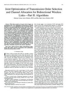
Assuming the leakage flux in the magnetic shell and air is negligible, then the magnetic flux produced by the primary winding can be divided into three paths. The first path passes through the airgap of the endfaces of the magnetic core and the magnetic shell, this is called the main flux q50. The second path passes through the airgaps of the magnetic core sides, facing the two secondary windings and the magnetic shell, this is called the secondary side flux &. The last path passes through the airgap of the magnetic core side, facing the primary winding and the magnetic shell, this is called the main side flux &. The structure of the solenoid LVDT and the magnetic fluxes are shown in Fig. 1. As shown in Fig. 1, a primary coil of length h,, two identical halves of a secondary coil of length h2, outside radius of coils D,outsiide radius of magnetic core d, the depths of the shell inserting two secondaries are denoted as t , and t2, and the airgaps of the shell sides are represented as a1 and 6,. The solenoid LVDT is a symmetrical structure. In Fig. 1, q5,, is comprised of $ooland $oo2.Similarly, is and comprised of and $(.,. q5m is comprised of $"2. Based on the magnetic flux, the equivalent magnetic circuit for an LVDT can be illustrated as Fig. 2, where the magnetomotive force (MMF) and Go,, Cy,, Gml, GO2,Gs2and Gm2are the magnetic conductances of the relative magnetic fluxes. 189

the magnetic conductances can be approximately determined by:

Go1 = PonR2/S1

(1)

Gs1 = (h2 - 61)g Similarly, for GO2and Gs2

(2)

Go2 = POTR2/62

(3)

Gs2 = (h2 - 6 2 ) g (4) Where R is the flux effective radius determined by the magnetic-core radius and its airgap in the endside; g is the specific magnetic conductance between cylindrical surfaces which can be obtained from 2,u0x/1n(D/d) [2]; is the air permeability. In Fig. 2, G,, and Gm2can be calculated from eqn. 5:

A I

I

Fig. 1 Structure of solenoid LVDT and the magnetic jluxes Magnetic fluxes: Qoj = main path; $s, = secondary sidepath; dml= main sidepath; Qm2 = main sidepath; @,2 = secondary sidepath; $oz = main path

d d m l x = FxdGm1x (5) At different positions of the windings, the magnetomotive force Z,N, and the crossing number of turns in the windings passed by the flux will be different. The magnetomotive force for an offset x from the centre (see Fig. 3) of the primary winding is given by

F, = I I N , = I1NiX/hl (6) Where 11 is the primary current and N I represents the number of turns in the primary windings. Using eqn. 6,

=i

h1/2

4ml

F 11. NI.

d4mlx

1

h1/2

xdx

= (IINlg/hl)

(7)

= I1N1gh/8

Thus,

Gm1 = $ m l / ( I l N l )

gh1/8

1

(8)

Similarly, Fig.2

Equivalent magnetic circuit of an LVDT

Gm2 gh2/8 (9) After different magnetic conductances are calculated, the total magnetic conductance of the magnetic circuit of the primary winding, its self-inductance L and flux @ can be computed using the following equations: G = (Go1 + Gs1+ Gm1)//(G02+ Gs2 + Gm2)

L

=N,~G

4 = IiNIG

(10)

(11) (12)

2.2 Mutual inductance The main sideflux @m that does not cross the secondary windings, is not able to produce mutual inductance, but the main flux q50 which crosses all the secondary windings will produce the main mutual inductance Mol and MO2.The calculations for the main mutual inductance can be obtained using the equations as follows: Qoi

Fig.3

Mol

Calculation of the main magnetic conductance

N2401

1

N2IiNiGoi/2

Q ' O I / ~ I = N2NiGo1/2

1

(13)

Similarly,

2.1 Magnetic conductance Normally, the magnetic reluctance of magnetic materials is much lower than that of an airgap of the same dimensions, and, therefore, the magnetic reluctance of magnetic materials can be neglected. If this is the case, 190

MO2 = N2N1Go2/2 (14) Where N2 is the number of turns in the secondary windings. The secondary side flux &, which crosses parts of the secondary windings, produces side mutual inductances IEE Proc -Sei Meas Technol, Vol 144, No 4, July 1997

M,, and Ms2. The calculation of the side mutual inductances is illustrated in Fig. 4.

series opposition, then the output voltage can be described as

Eo = (M1- M 2 ) E l / L (19) Eqn. 19 is derived from equation 4.46 given by PallasAreny and Webster [l]. Therefore, Eo = ENzg(2: - t : ) / ( 4 h ~ N l G ) Because of the symmetrical structure,

Go1 = Goa;

4 Tt 1

dQslz

1

tl

= (IiNlNzg)/(’&)

xdx

= 11 NIN2 gt: / (4hz)

Msi = ‘@si/Ii = N1”2&/(4h2)

(15)

Similarly, Ms2 = N1N2gt;/(4h2) (16) The mutual inductance M I produced between the primary winding and the upper secondary winding can be given by eqn. 17 and the mutual inductance M 2 produced between the primary winding and the lower secondary winding can be given by eqn. 18:

+ Msi = N2N1(poi7R2/(2bi)+ g t ; / ( 4 h 2 ) ) (17)

Mz = Moz

+ Ms2 = N2Ni(poi7R2/(2&)+gti/(4hz)) (18)

Where the flux effective radius R is decided by the airgap 6 (6 = h - t ) and the diameter d of the magnetic core When 6 is changed slightly by a displacement, then R will change accordingly in the same direction. If the measuring displacement is small, p00“R2/(26,) and ,4@2/(2S2) are not considered to change. Therefore, one conclusion can be drawn, namely that the main mutual inductance does not change when the movement produces a small displacement.

2.3 Output voltage and sensitivity of transducer The primary winding is excited by a voltage E , vvith an excitation frequency f (the resistance losses can be considered negligible). If there is no load connected to the secondary and the secondary windings are linked by IEE P r o c S c i . Meas. Technol., Vol. 144, No. 4, July 1997

(22)

Experimental results

3

tl

Mi = Mol

- At

K = Eo/At = El N 2 g t o / ( h ~ N l G )

The differential flux linkage at the position x, offset from the intersection point of the primary winding and the secondary windings (see Fig. 4), can be computed by dQs1z Nzd4slz Where N , = Nzx/hz and d 4 s l , = IiNlgdx/2 Therefore d q s l z = (IlNlN2gzdx)/(2h2) =

to

Eo = EiN2gtoat/(h2NlG) (21) The sensitivity of the transducer can be determined by

Side mutual inductances

*si

tl

Where to is the height of the magnetic core inserted into the secondary windings with the core being put in the centre of the primary winding. Therefore,

62

Fig.4

ti = to + At;

(20)

Based on the equations given in the preceding text, the experimental tests on the output voltages and sensitivities have been used for different LVDTs. The structure parameters of one of the tested LVDTs are as follows: d = 3mm, D = 9mm, hl = h2 = 4mm, to = 2mm, the spacing between the coils is 2mm, the length of the magnetic core is lOmrn, N I = N 2 = 1000, E = 3 V , f = 1000Hz. To identify the given algorithms and eddy-current effect, two tested transducers with the same structure parameters have different magnetic materials for magnetic core and magnetic shell. For different displacement, the test output voltages and calculation values are shown in Table 1, where test voltage 1 is the output voltages of one transducer with magnetic material of nickel-iron (Fe-Ni) alloys and test voltage 2 is the output voltage of another transducer with magnetic material of ferrites. Table 1: Calculation and test results of LVDT output voltage (in mV)

wm

Displacement,

Calculated voltage

-500

Test voltage 1

Test voltage 2

-250.15

-258.19

-254.78

-400

-200.13

-207.70

-204.12

-300

-150.09

-155.21

-153.07

-200

-100.06

-102.92

-101.98

-1 00

-50.03

-51.35

-51.33

0

0.00

2.05

-0.82

100

50.03

52.17

50.24

200

100.06

103.86

100.76

300

150.09

156.04

151.36

400

200.13

208.93

202.45

500

250.15

258.97

253.70

It can be seen that the big difference between the calculated and test values; is due to the zero position and the large displacement. For the zero position, the difference is caused by residual voltage of no absolute symmetrical structure such as size and material consistency. For the large displacement, the errors come from the approximation of the flux effective radius and leakage. Different magnetic materials achieve different sensor sensitivity because of permeability and eddy-current 191

losses. With the two magnetic materials, nickel-iron (Fe-Ni) alloys have higher permeability with higher eddy-current losses; inversely, ferrites have lower permeability with lower eddy-current losses. Therefore, the effect of different materials is not significant. More test data can be found in Tian and Zhang [5]. From Table 1, the error of the output voltage against the theoretical calculations discussed here are found to be below 5%. Conclusions

4

There are many advantages to using LVDTs, they have total electrical isolation and are contactless devices, so frictioned effects and wear are minimal. They have high repeatability, especially of the zero position, due to their symmetry, They have directional sensitivity, high linearity, high sensitivity and a broad dynamic response. Compared with the conventional method that the sensitivity depends on the excitation frequency, the alternative algorithms that the sensitivity does not depend on the excitation frequency has been provided and tested in this paper. The results have provided a systematic explanation of the research findings reported by Saxena [6] and Kano [7]. The calculation method and equations can be used for designing LVDTs. Based on the given algorithms, the comparison between solenoid LVDTs and solenoid differential inductive transducers can be shown as follows: By a similar method, the self-inductance given by Zhang [8], for the solenoid differential inductive transducers, is L=L,+L,

+

= N2(p07rRR2/6 gt3/(3h)) Where L,%is the main self-inductance and L, is the side self-inductance. The mutual inductance of LVDTs is

M = MO

192

+ M s = N21V,(po7rR2/(26)+9t2/(4h2))

Both are composed of two parts, the first part is roughly constant and the second part is L,.-t3 and M, -t2. Therefore, it can be seen that the linearity of LVDTs is better than that of the solenoid differential inductive transducers, and LVDTs have longer measuring ranges and are widely used. Eqn. 22 shows that increasing the number of turns of the secondary windings and decreasing the secondary windings can help in achieving highly sensitive LVDTs. LVDTs are well known and well established transducers, the algorithms given in this paper are useful for new transducer design and calculation as a simple engineering computing method under the current status of no more effective methods for the transducer. As we can see, the algorithms are not highly accurate and fail to take account of eddy-current effects. To increase the accuracy, further work will carry on the nonlinear magnetic flex modules and finite-element methods for computing eddy-current problems. References PALLAS-ARENY, R., and WEBSTER, J.G.: ‘Sensors and signal conditioning’ (Wiley-Interscience, 1991) NEUBERT, H.K.P.: ‘Instrument transducers - An introduction to their performance and design’ (Oxford University Press, 1975, 2nd edn.) YU, H.T., SHAO, K.R., and LAVERS, J.D.: ‘A finite-element method for computing 3D eddy-current problems’, ZEEE Trans. Magn., 1996, 32, ( 5 ) , pp. 43204322 PARK, I.H.: ‘Design sensitivity analysis for transient eddy-current problems using finite-element discretization and adjoin variable’, ZEEE Trans. Magn., 1996, 32, ( 3 ) , pp. 1242-1245 TIAN, G.Y., and ZHANG, N.: Research report, 1994, Chengdu University of Science and Technology, People’s Republic of China SAXENA, S.C., and LAL SEKSENA, S.B.: ‘A self-compensated smart LVDT transducer’, ZEEE Trans. Instrum. Meas., 1989, 38, pp. 148-153 KANO, Y., HASEBE, S., HUANG, C., and YAMADA, T.: ‘New type linear variable differential transformer position transducer’, ZEEE Trans. Instrum. Meas., 1989, 38, pp. 407409 ZHANG, N.: ‘A calculation of solenoid differential inductive transducers’, Chin. J. Sei. Instrum., 1989, XI, (3)

IEE Proc.-Sei. Meas. Technol.,Vol. 144, No. 4, July 1997