initially looked promising has been found to be less promising after being partially ...... [15] Durfee, Edmund and Victor Lesser, âIncremental Planning to Control a ...
Blackboard Systems for Knowledge-Based Signal Understanding Norman Carver and Victor Lesser
A sophisticated signal understanding system requires knowledge-based interpretation techniques as well as sophisticated signal processing techniques. Blackboard systems are the most widely used artificial intelligence (AI) frameworks for understanding and interpretation problems. This paper reviews the blackboard model of problem solving and discusses how blackboard systems can be used for understanding problems. However, it does not specifically show how blackboard systems can be used for knowledge-based signal processing. Integration of signal processing and understanding via blackboard systems is addressed in [35]. We use the term signal understanding rather than signal processing here, because our focus is on the development of “high-level” descriptions of data in terms of the “situations” it represents. Another way of saying this is that signal understanding involves the meaning of the data, while signal processing is generally limited to the extracion of important features—i.e., semantic versus syntactic descriptions. The notion of understanding has also been associated with enabling a system to act on the data in an appropriate manner. Thus, a sound understanding system must do more than just identify harmonically-related acoustic signals, it must also determine their source—e.g., a ringing telephone (that may need to be answered). Likewise, a radar understanding system must do more than just identify echoes, it must also be able to explain the echoes in terms of the movements of certain vehicles, environmental disturbances, and so on. Signal understanding problems cannot typically be solved by applying the kind of algorithmic data transformations used in traditional signal processing. This is because signal understanding applications often involve a great deal of underlying uncertainty: critical features cannot be accurately or precisely “extracted” or with the types of features that can be extracted the space of situations to be considered is still very large. For example, while there may be models of the output that individual sources/targets should ideally elicit from a sensor, it may not be possible to have exact models for the interactions of every possible combination of sources. Add to this the uncertainty over the effect that environmental conditions or other phenomena may have on the sensor output and the problem is very difficult to solve algorithmically. Blackboard systems (and AI techniques in general) are appropriate for understanding problems that involve very large answer spaces as well as uncertain, errorful, or incomplete data and problemsolving knowledge. These characteristics can produce a combinatorial explosion in the number of situation models that must be considered (this issue is pursued further in Section 1). Solving such problems requires an approach that is very different from the algorithmic approaches of traditional signal processing. Instead of attempting to directly determine the best complete answer, in blackboard-based problem solving partial possible solutions are incrementally constructed and
1
refined as part of a search process. In such a process, the data (which may have already undergone algorithmic signal processing) is first examined to try to produce likely partial models. These preliminary potential models drive further processing, influencing decisions about the best models to pursue and the best ways to pursue them (they may also influence parameter settings for further algorithmic signal processing). In other words, instead of trying to develop a single strategy that is appropriate for all situations, a blackboard system is structured so that it is able to adapt to specific situations by opportunistically selecting among a large set of diverse problem-solving methods. This requires a system with a great deal of knowledge and flexibility. For instance, significant amounts of task-specific heuristic control knowledge must be encoded and applied in order to decide what to do next—to constrain the search and limit the portion of the answer space that must be examined. The paper begins with a section that identifies signal understanding as an example of a class of artificial intelligence problems called sensor interpretation problems. The next section introduces the blackboard model of problem solving and discusses why it is appropriate for signal understanding problems. The third section presents an example aircraft monitoring application to demonstrate how blackboard systems can be used for interpretation problems. Section four expands on the example by discussing the issues that affect the structuring of interpretation problems and problemsolving knowledge. Section five examines the critical issue of control in blackboard systems. It begins with an introduction to the major issues that are relevant to the control of blackboard systems and then examines several of the control schemes that have been developed for blackboard systems. The paper concludes with a summary of the major points and a discussion of current blackboard systems research that is relevant to signal understanding.
2
Attack Mission
Recon Mission
Transport Mission
XXX y : �� XX6 ��� Track
6 Acoustic Ghost Track
6 Acoustic Ghost Sensor Malfunction
: � ��� � � � ��
Acoustic Group
XXX y : �� XX� 6��
Vehicle
BM
Acoustic Noise
Acoustic Signal
XXX y XX6
Acoustic Data
B
B B
B
B
B
B
B�
* � �
Radar Ghost
Radar Data
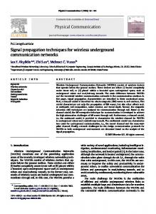
Figure 1: Interpretation type hierarchy for example aircraft monitoring application.
1
Signal Understanding as Interpretation
Signal understanding is one example of a class of AI problems often referred to as sensor interpretation problems. Interpretation involves the determination of high-level, conceptual explanations of sensor and other observational data. The interpretation process is based on a specification of the relations between the data types and a set of abstraction types. These types form a hierarchy like the one for an example aircraft monitoring system shown in Figure 1. An interpretation system analyzes the available data and creates hypotheses that provide possible explanations for subsets of the data. Each hypothesis represents a possible instance of its associated interpretation type. Higher-level hypotheses are said to explain lower-level hypotheses while, conversely, lower-level hypotheses are said to support higher-level hypotheses. Answers are typically in terms of top-level type hypotheses since these types represent the most abstract and most encompassing level of explanation for the data. The lowest levels (i.e., the leaves) of the hierarchy represent the data upon which the interpretation process will be based.1 Each interpretation type has a set of “attributes” and hypotheses include corresponding slots. The relations between the types define certain constraints on the acceptable values of these slots. Thus, the creation of relations between hypotheses requires that these constraints be checked. In other words, the slots of lower-level hypotheses must meet certain constraints in order to create a particular type of higher-level hypothesis as a potential explanation of the lower-level hypotheses. The slot values of the lower-level hypotheses also define the slot values of consistent higher-level hypotheses. In the aircraft monitoring example of Figure 1, data from acoustic and radar sensors (i.e., Acoustic Data and Radar Data) is abstracted and correlated to identify potential aircraft sightings 1
Note that data types may feed into the hierarchy at different levels. Here Radar Data immediately provides support for Vehicles, while Acoustic Data must be abstracted to get to the Vehicle level. Likewise, it would be possible to have intelligence reports or other kinds of evidence that could provide direct evidence for Mission-types.
3
(Vehicle hypotheses), movements (Track hypotheses), and goals (Mission hypotheses) that might explain the sensor data. Each abstraction level represents the application of additional constraints. For instance, Track hypotheses must have particular vehicle ID and movement slot values in order to be able to be consistent with each particular Mission explanation. A Track’s slot values are defined/constrained by the slot values of its supporting Vehicle hypotheses which are in turn defined by the slot values in their supporting data or hypotheses. Besides the top-level Mission types, the hierarchy includes other top-level types—like Acoustic Noise—that are not of interest as answers. These “nonanswer” types are useful for interpretation because they can provide alternative explanations for the data. The blackboard system example in Section 3 includes further explanations of the abstraction types in Figure 1. Interpretation is based on the notion of abduction: if B types cause A types, then when an A is observed we might infer (hypothesize) a B as an explanation for the A. Likewise, given a possible B, in order to provide support for the B we can look for an A instance that the B should have caused. An interpretation type hierarchy like that in Figure 1 can be viewed as a causal hierarchy. For example, an aircraft on a certain Mission will cause the aircraft to travel a Track with certain attributes. This eventually causes acoustic signals with certain attributes, causing the acoustic sensor to produce corresponding data (the reasons why we do not want to go directly from the top-level types to the data are discussed in Sections 3 and 4). The distinction between the explanation and causal views of the type relations is analogous to the difference between analytic and generative models [37]. Abductive inferences are uncertain; while plausible, they are not logically correct. Abductive inferences are uncertain because there can be multiple causes (and thus multiple possible explanations) for data and hypotheses. For example, it may be that both B and C types cause A types and that there is a C instance that is the true cause (explanation) for the A mentioned above. This potential for alternative explanations for data and hypotheses is the primary source of uncertainty in interpretation inferences (and thus interpretation hypotheses). However, besides this uncertainty inherent in abductive inferences, a number of other factors can contribute to uncertainty about the correctness of interpretation hypotheses. For example, because of sensor resolution limitations, data attributes like position and frequency class may be imprecise. As a result, the validity as well as the correctness of interpretation inferences may be uncertain (since it may not be possible to say the data conclusively meets the necessary interpretation constraints). Also, sensors may malfunction, causing events in the environment to be missed or data to be produced for nonexistent events. Because abductive inferences are uncertain, interpretation hypotheses are uncertain and the primary goal of an interpretation system is to resolve its hypothesis uncertainty sufficiently to produce acceptable answers. There are are two main techniques resolving hypothesis uncertainty: incremental hypothesize and test (also known as evidence aggregation) and differential diagnosis. Incremental hypothesize and test means that when a hypothesis has only partial support evidence, the system should attempt to find the complete support that the hypothesis would have if it were
4
correct. Differential diagnosis means that the system should attempt to discount the possible alternative explanations for a hypothesis’ supporting evidence. Hypothesis correctness can only be guaranteed by doing complete differential diagnosis—i.e., discounting all of the possible explanations for the supporting data. Even if complete support can be found for a hypothesis, there may still be alternative explanations for all of this support. However, while complete support cannot guarantee correctness, the amount of supporting evidence is often a significant factor when evaluating the belief in a hypothesis (this is the basis of hypothesize and test). For example, once a Track hypothesis is supported by correlated sensor data from a “reasonable” number of individual positions (Vehicle hypotheses), the belief in the Track will be fairly high regardless of whether alternative explanations for its supporting data are still possible. Blackboard systems typically have been limited to hypothesize and test strategies because of the characteristics of their evidence and control frameworks (and because interpretation problems require constructive problem solving—see below). This issue will be discussed further in Section 5.5. In order to determine whether hypotheses are sufficiently certain and to make control decisions about the hypotheses to work on next, an interpretation system must be able to represent the level of uncertainty in its hypotheses. Hypothesis uncertainty is typically represented by attaching numeric “ratings” to the hypotheses when they are created or modified. However, the rating schemes use in most blackboard-based interpretation systems have been ad hoc—i.e., they have not used formal numeric representations of uncertainty (like probabilities) and they have not accurately treated interpretation inferences as abductive inferences. The development of techniques for reasoning about uncertainty is a major area of research in AI (see for example [8, 42]) and is beyond the scope of this chapter. While hypothesis uncertainty is an important issue, the key reason why interpretation problems require AI techniques is that solving them generally means a search process. The reasons for this were discussed in the introduction to this chapter. However, in order to better understand what makes these problems special, it is necessary to understand the differences between interpretation problems and similar problems that can be solved with classification techniques. Clancey [6] distinguishes between two classes of problem solving: classification problem solving and constructive problem solving. In classification problem solving, the problem solver selects “the answer” from among a pre-enumerated set of possible solutions. “Classification problems” may sometimes be solved through pattern matching: comparing an object (or a processed representation of the object) against a set of templates and picking the “best match.” This sort of approach has been used for isolated word recognition [44]. For “classification problems” in which evidence must be aggregated to make a selection, there are well-developed numeric evidential reasoning techniques like the Dempster-Shafer calculus and Bayesian networks [42] that can be used. For example, simple medical diagnosis problems[1, 43] can be solved by entering evidence into a belief network (of findings and diseases) until the answer (the diagnosis) can be identified with sufficient certainty [42, 43] (though determining the best evidence to gather may be critical to acceptable performance in such systems).
5
In constructive problem solving, both “the answer” and the set of possible solutions are determined as part of problem solving. Constructive problem solving is required when the set of possible solutions cannot be enumerated prior to problem solving. Interpretation problems generally require constructive problem solving because of the combinatorics of their answer spaces [2]. For example, in aircraft monitoring, an (effectively) infinite number of different Track hypotheses (possible aircraft movements) must be considered for each potential aircraft and an indeterminate number of Track hypotheses may be correct since the number of aircraft that will be monitored is unknown. The possibility of multiple aircraft also produces a combinatorial number of data combinations that may have to be considered due to “correlation ambiguity” [29]. Formal numeric techniques like the Dempster-Shafer calculus and Bayesian networks are often not directly applicable to constructive problem solving because they require a complete “frame of reference.” Thus, in at least one sense, interpretation problems are more difficult than classification problems. In fact, constructive problem solving requires numerous capabilities that are not required for classification problem solving. For instance, constructive problem-solving systems must be able to represent incomplete and imprecise hypotheses, incrementally create and extend such hypotheses, maintain large numbers of these hypotheses, and apply significant amounts of knowledge to focus the construction process (i.e., control the search for the answers). This last point is critical because a combinatorial number of hypotheses may be able to be created to explain the data, creating each hypothesis may be computationally expensive, and a variety of methods may be used to resolve the uncertainty in each of them. The distinction between classification and constructive problem solving is also relevant to understanding why blackboard systems have typically relied on hypothesize and test strategies. Differential diagnosis requires an understanding of the possible alternative interpretations for the supporting data of a potential answer hypothesis. This is relatively straightforward in “classification problems” since the set of alternatives can be fully enumerated. In order to apply differential diagnosis techniques to “constructive problems,” more sophisticated methods for representing and evaluating alternatives is required (see Section 5.5) because the alternatives cannot be fully enumerated.
6
2
Blackboard Systems
Blackboard systems are the most used artificial intelligence architectures for sensor interpretation and related problems (see, for example, [4, 15, 29, 30, 32, 36, 38, 40, 45]). This section introduces the blackboard model of problem solving and examines the major elements of a basic blackboard architecture. Section 3 uses an aircraft monitoring example to make the concepts presented here more concrete. Sections 4 and 5 expand on the issues involved in implementing an interpretation problem using a blackboard framework. The concept of a blackboard system originated with the Hearsay-II speech understanding project [18, 30, 31, 41]. Understanding connected/continuous speech is a difficult problem. It involves the kinds of uncertainties and combinatorics that were discussed in the chapter introduction and Section 1: variability in the speaking process of different people, environmental noise and distortions in the sensing process, incomplete/imprecise models of speech, combinatorial explosion of model interactions (e.g., co-articulation phenomena result in words “looking” different depending on the adjacent words), and so on. This means that the speech understanding problem cannot be solved using classification techniques like template matching (though this can succeed for the recognition of isolated words). Understanding connected speech requires a search process that generates and evaluates numerous uncertain, partial solutions. The Hearsay-II group came up with a system based on the following idealized model of problem solving: a group of experts sits watching solutions being developed on a blackboard and whenever an expert feels that he can make a contribution toward finding the correct solution, he goes to the blackboard and makes appropriate changes or additions. The first thing to note about this idealized model is that it is very different from the highly structured and deterministic model that underlies standard computer programming languages. In the blackboard model, there is no predetermined order in which the experts apply their knowledge and no predetermined order in which data/hypotheses are pursued. Among the key ideas behind this idealized model are that problem solving should be both incremental and opportunistic. That is, solutions should be constructed piece by piece and at different levels of abstraction, basing the selection of the methods to be used on the data that is available and on the intermediate state of the possible solutions. Solutions are constructed using an “island driving” strategy: hypotheses that are judged to be likely (“islands of certainty”) are incrementally abstracted and extended to produce a complete final solution. This opportunistic strategy allows the system to work where it can make the best progress instead of being limited to a fixed, predetermined strategy that may not be best for every problem situation. In speech understanding, for example, well-sensed words can constrain the search for poorly sensed words—as compared with a fixed beginning to end strategy. Other key ideas behind the model are that problem-solving knowledge should be partitioned into a set of independent modules and that alternative solution hypotheses should be contained in an integrated, global database. In conventional algorithmic problem solving, a single algorithm/program encodes all of the knowledge needed to solve the problem. This makes it difficult to change the control strategies and the methods for solving (particular aspects of) the problem. Partitioning the 7
Knowledge source ("Expert")
Blackboard
Knowledge source ("Expert")
Data (there is no control flow in this model) Figure 2: The idealized blackboard model. problem-solving knowledge into a set of independent modules (the “experts”) provides the system with the flexibility to experiment with alternative control strategies and alternative problem-solving methods. The ability do this kind of experimentation is crucial for the successful development of knowledge-based systems. An integrated, global database permits module independence because it assures that modules can recognize when they should be invoked without requiring the modules to directly invoke each other. In addition, because there is a single integrated representation of all the developing solution hypotheses, it is possible to have multiple, alternative solution paths being pursued in parallel and to be able to recognize the relationships among the paths. We will now look in more detail at the architecure of blackboard systems. Any problem-solving architecture must prescribe methods for structuring and using three major components: domain knowledge, a database, and control knowledge. Domain knowledge consists of the task-specific knowledge and procedures that are used to actually solve the problem. The database holds the initial data, intermediate results, and the answer. Control knowledge includes both task-specific and task-independent knowledge about how/when to use the domain knowledge to best solve the problem. The basic blackboard problem-solving model prescribes a database structure and domain knowledge interaction protocols, but says little about control knowledge (control is discussed further in Section 5). A blackboard system is composed of two main components: the blackboard and a set of knowledge sources (or KSs). Figure 2 shows the relationships between these components. The blackboard is a shared, global database that contains the data and the developing hypotheses. The knowledge sources contain the domain knowledge of the system (they are the “experts” of the idealized model described above). KSs examine the blackboard and construct new hypotheses or modify existing hypotheses when appropriate. The knowledge sources are intended to be totally independent (modular): their execution should not explicitly depend on the execution of other KSs and they should not communicate directly with 8
each other. In the blackboard model, sequencing of KSs and communication between KSs occur only via the creation and modification of hypotheses on the blackboard. For example, a knowledge source that created an Acoustic Signal hypothesis from a piece of Acoustic Data (see Figure 1) would not directly call the knowledge source that abstracts this hypothesis to create an Acoustic Group hypothesis. Instead, the Acoustic Signal to Acoustic Group KS would see the creation of an Acoustic Signal hypothesis on the blackboard and recognize that it could now apply its knowledge. In addition to being a global database, the blackboard model prescribes that the blackboard be structured as a hierarchy of spaces (also often referred to as levels). Each space should represent a different level of abstraction or a different point of view on the data and problem solution. Only particular types of hypotheses are allowed in each space. For interpretation problems, the set of blackboard spaces would correspond to the levels in the interpretation type hierarchy (Figure 1). Decomposing the blackboard into spaces (with corresponding hypothesis types) serves two related functions: it facilitates the incremental construction of solutions and it helps to partition the domain knowledge into KSs. Section 4 discusses the issues involved in structuring problems when using blackboard systems. Blackboard spaces are themselves structured in terms of a set of dimensions. Each space has its own particular set of dimensions that depend on the slots in the types of hypotheses that can be placed into the space. Typically, each space in a blackboard will include one or more dimensions that are common to all of the spaces. For example, in the aircraft monitoring example of Figure 1 (see also Section 3) all of the spaces include time, X, and Y dimensions. Additional dimensions may be specialized to the particular space—e.g., group-class in the Acoustic Group space of an aircraft monitoring system. Dimensions are used to define the “location” of a hypothesis within a space in order to provide efficient associative retrieval of hypotheses. Event-directed or data-directed KS invocation means that KSs must evaluate hypothesis characteristics such as whether there are hypotheses that are “close” to a triggered hypothesis or are within a certain “region” of a space. For example, a KS for extending a Track hypothesis by adding another Vehicle support (see the example in Section 3) would have to check if a Vehicle hypothesis exists for the right time and the right region of space to determine if it is applicable. Retrieval efficiency is an important issue for blackboard systems because of the large numbers of hypotheses they must often deal with and because of the datadirected invocation of knowledge sources. The representation of hypotheses on the blackboard is termed “integrated” not only because of the global nature of the blackboard, but also because each hypothesis is kept linked to the hierarchy of hypotheses and data that represent the support and possible explanations for the hypothesis. This hierarchical structure can be used to determine the relationships between any two hypotheses. For instance, it can be used to determine that two hypotheses are competing alternatives and can show exactly why this is so (in terms of shared supporting data or hypotheses). An example of this sort of structure can be seen in Figure 10 in Section 3. This integrated approach to representing hypotheses can be contrasted with the “possible worlds” approaches of Truth Maintenance
9
Systems [3] which make it difficult to understand in detail the relationships between alternative hypotheses. The idealized blackboard model does not prescribe any particular control framework: whenever a KS can contribute to the developing solutions, it immediately does so. Thus, knowledge sources must not only know how to create or modify hypotheses as part of constructing a solution, they must also be able to recognize when they can take these actions. For this reason each KS consists of two functional components: the precondition and the action. The precondition portion examines the state of the blackboard in order to determine if the action portion is applicable (as was discussed earlier in the context of associate retrieval of hypotheses). If it is, the precondition portion can then create an instantiation of the action portion in terms of the relevant blackboard objects. Despite the appeal of not having to specify control strategies, there are two problems with the idealized blackboard model. The first problem is that most computers have had a single processor. Having a single processor means that KSs can actually only be executed one at a time (in effect, only one “expert” can be at the blackboard at any time). The second problem with the lack of control in the idealized blackboard model is that blackboards are typically applied to combinatorially explosive problems (like signal understanding and other interpretation problems). In such problems, computation time considerations make it undesirable or even impossible to execute all of the KS actions that are possible before an acceptable answer is found. Executing actions that create and pursue unlikely hypotheses “distracts” the system by forcing useful actions to compete with nonuseful actions for resources. This can greatly delay the construction of the final answers. These problems suggest that a control mechanism that can help to focus the search for the answers must be added to the blackboard model presented so far. In effect, the idealized model must be modified so that the experts raise their hands when they can contribute something and someone else then decides whether their contributions are likely to be useful or not. This allows the system to focus its attention on the most promising partial solutions in order to make the best use of its limited resources and produce answers more quickly. Focus-of-attention is a critical issue for most blackboard applications and it has been the subject of much of the research on blackboard frameworks. Control issues will be pursued further in Section 5. To handle the control problems just discussed, Hearsay-II used an agenda mechanism: all potential actions are placed onto a scheduling “queue” where they are rated and selected for execution by the scheduler. The basic Hearsay-II architecture is shown in Figure 3. This agenda-based control approach has been followed in most subsequent blackboard systems. Thus, the Hearsay-II architecture as shown is the prototypical blackboard architecture. When reference is made to a standard, data-directed blackboard system, a system with this basic Hearsay-II architecture is meant. Having just referred to Hearsay-II as a data-directed blackboard system, it is important to point out that complex interpretation problems require the integration of both data-directed and goaldirected control factors. Our description of Hearsay-II as a data-directed system is a simplifying abstraction of the Hearsay-II implementation that makes clear the key elements of a data/eventdirected blackboard system. Hearsay-II actually made use of a number of additional features that
10
... Knowledge Sources
Blackboard
...
Events
Blackboard Monitor Data Control
Agenda KSIs
Scheduler Focus-of-control Database
Figure 3: The data-directed, agenda-based blackboard architecture. allowed it to integrate goal-directed factors into the control decisions.2 These features will be noted and discussed as appropriate in the following sections. Section 5 in particular will show how many of these features have been formalized or generalized in later blackboard frameworks. Another problem with the idealized blackboard model is that checking the preconditions of every KS after each action is taken could become very expensive. Because of this, the blackboard model of Figure 3 includes a mechanism for limiting the checking of KS preconditions. All changes to the blackboard are categorized in terms of a set of blackboard event types. Every time a KS action is executed, the changes to the blackboard are described in terms of the blackboard event types. These events descriptions are passed to a blackboard monitor that uses a table of the KSs that are interested in each event type to identify those KSs whose preconditions should be checked (i.e., that should be “triggered”). Figure 4 summarizes the main control loop in a data-directed blackboard system. As we have just said, every time data is inserted onto the blackboard or hypotheses are created or modified, a description of these changes in terms of blackboard event types is passed to the blackboard monitor. The blackboard monitor identifies those KSs that might be interested in the particular blackboard events and causes the preconditions of these KSs to be checked.3 Instead of executing a KS action 2
For example: prediction KSs, policy KSs, and focus-of-attention data. In early verions of Hearsay-II, once a KS was triggered, the precondition procedure was placed onto the agenda instead of immediately being executed. This made it possible for the execution of preconditions to be controlled by the scheduler. BB1 uses a similar approach to implement precondition-action backchaining (see Section 5.4). 3
11
KS ACTION COMPONENT: Execute KSI Selected KSI
Blackboard Events
BLACKBOARD MONITOR: Identify Triggered KSs
SCHEDULER: Rate KSIs and Select KSI for Execution
Updated Agenda
Triggered KSs and Triggering Events
BLACKBOARD MONITOR: Update Agenda with KSIs Representing Activated KSs
KS PRECONDITION COMPONENTs: Check Preconditions of Triggered KSs
Stimulus and Response Frame Info from Successful KS Preconditions Figure 4: The control loop for the data-directed, agenda-based blackboard architecture. as soon as it is found to be applicable, a successful precondition produces a knowledge source instantiation (KSI)4 and places it onto the agenda (the scheduling “queue”). Each KSI represents an action that could potentially be taken by the system and includes the hypothesis bindings and other information necessary to execute the KS action. Thus, at any given time, the set of KSIs on the agenda represent the actions that the system could take next. Once the triggered preconditions have all been checked and any new KSIs placed on the agenda, the scheduler selects the KSI to be executed next, removes it from the agenda, and executes it.5 Execution of a KSI can result in However, these capabilities came at the cost of a much more complicated scheduler and were not ultimately useful given the level of the knowledge available to control their useage. 4 Knowledge source instantiations are also sometimes referred to as knowledge source activation records (or KSARs). 5 Actually, before a KSI can be executed, the system must verify that it is still applicable. Because there can be a delay between when a KS’s precondition is checked and when the resulting KSI is executed, the situation on the blackboard may have changed so that the KSI is no longer applicable. Reverifying KSIs has been handled in several ways, ranging from simply re-executing the precondition procedure of the KS to specifying “obviation conditions” [22]
12
the creation or modification of hypotheses bringing the system back to the beginning of the control loop. Since it is the scheduler that selects the next action to take, it is the scheduler that determines the focus-of-attention in a blackboard system. The scheduler selects the next KSI to execute by calculating a rating for every KSI on the agenda and choosing the highest rated KSI. Thus, the scheduler’s KSI rating function embodies the strategy (control) knowledge of a blackboard system. KSI ratings are typically based on factors like the ratings of the hypotheses that triggered the creation of the KSI and the “desirability” of creating the hypotheses which the KSI should create. We will look at ratings further in Section 3 when we look at an example blackboard-based aircraft monitoring system. The blackboard control cycle repeats until acceptable answers have been found or else there are no KSIs on the agenda. Determining whether acceptable answers have been found is known as the termination problem. Termination can be difficult and it will be examined in Section 5.
with each KS. Obviation conditions allow the system to recognize when KSIs are no longer applicable so that they can be removed from the agenda as soon as possible.
13
3
An Example: Aircraft Monitoring
In this section we present a short example to show how a blackboard system may be used to implement the understanding portion of an aircraft monitoring application. Further details about this and related vehicle monitoring applications can be found in [3, 10, 32]. We will concentrate here on the basic, data-directed blackboard framework described in the previous section. The example will also be discussed in the succeeding sections of this chapter in the context of more detailed explanations of the structuring and the control of blackboard problem solvers. As we have said, the interpretation process involves the incremental construction and extension of hypotheses representing possible partial solutions. The interpretation hierarchy for our example aircraft monitoring application was shown in Figure 1. In the aircraft monitoring hierarchy of Figure 1, there are two types of data (Acoustic (sensor) Data and Radar Data) and three top-level Mission types that represent the possible purpose of aircraft movements. However, for this short example, only Acoustic Data will be used and answers will be restricted to the Track level. Acoustic Data and Radar Data are correlated at the Vehicle level. Vehicle hypotheses represent potential “sightings” of aircraft. Vehicle hypotheses include a position slot that is the point in space and time where the aircraft is hypothesized to be and an ID slot that identifies the type of aircraft. Track hypotheses represent the movements of aircraft over time. They must be supported by sequences of Vehicle hypotheses that could represent the movements of the same aircraft. Vehicle hypotheses must meet certain constraints to be able to support the same Track hypothesis: they must have consistent ID slot values and their positions must conform to the movement parameters of the particular type of aircraft represented by ID (e.g., maximum velocity). The Mission-level represents a further specialization of Track hypotheses in terms of the goal or purpose of aircraft movements. Mission-level hypotheses impose constraints on the ID of Tracks and on the permissible movements represented by the Track. The hierarchy may in fact be expanded further to the Scenario level (sometimes called the pattern level) in which Mission-level hypotheses from multiple aircraft are correlated to explain the overall goal of the individual aircraft Missions. Acoustic Data is interpreted through the Acoustic Signal and Acoustic Group levels to support Vehicle hypotheses. An Acoustic Signal hypothesis represents a single sensed acoustic signal in the environment and includes position and frequency-class slots. An Acoustic Group hypothesis represents a set of harmonically related acoustic signals that all emanate from a single mechanism on an aircraft. Thus, an Acoustic Group hypothesis will be supported by a set of Acoustic Signal hypotheses whose positions overlap and whose frequency-class slot values can be part of the same harmonic group. Acoustic Group hypotheses each include a position slot and a group-class slot that are defined by the values of the position and frequency-class slots of their supporting Acoustic Signal hypotheses. Since each aircraft typically has a number of mechanisms that generate acoustic signals, Vehicle hypotheses typically will be supported by several Acoustic Group hypotheses. In other words, the acoustic frequency spectrum created by an aircraft is not directly interpreted; the spectrum is first divided into appropriate Acoustic Groups. For this example we are assuming that only acoustic sensor data is available. The data is represented in Figure 5. The dots in the figure show the spatial orientation of clusters (spatially 14
1b
Ý 2b
Ý
Ú
×
Ú
6a
Ú
5a
Ö
3a
2a
1a
Ö
4a
× 5b × 6b
Y X
Figure 5: X-Y map of the clusters of acoustic data points for the example scenario. close groupings) of acoustic sensor data points. Associated with each dot is a label whose numeric portion denotes the time that the data was sensed—e.g., 1a data is from time 1. We are also assuming that the data point clusters can be used for indexing the data—having been created by automatic low-level routines. Being able to index the acoustic data via clusters is useful for focusing the search process since the data resulting from a single source tends to get clustered together (data points resulting from a single source may not end up with identical position attributes due to sensor imprecision and environmental disturbances). In this example we will make use of the clusters in certain “large-grained” KSs and for rating the data. Clustering can also be used as a type of approximate processing technique—see Section 5.3. Figure 6 gives the ratings that are associated with each data cluster (the relative size of the dots in Figure 5 reflects these ratings). Data is rated as it is placed on the blackboard. The data ratings are based on the loudness of the sensed frequencies and on the number of frequencies in the cluster. Since the data ratings influence the rating of data abstraction (synthesis) KSIs, the data rating scheme is intended to try to limit the processing of “noise” and to promote the use of “well-sensed” data from actual aircraft. The rating scheme used here is based on the following assumptions: noise is typically quiet relative to aircraft signals, noise typically has a sparse frequency spectrum relative to aircraft signals, and when the signals are louder they tend to be sensed with more precision (have less frequency-class and position uncertainty). Thus, the ratings are based on the average loudness of and the number of data points in the cluster. The situation that the data represents is that the “a” data has resulted from an actual aircraft, while the “b” data is “ghost” data that has resulted from environmental reflections. Ideally, data from an actual vehicle would be rated higher than ghost data. However, due to environmental disturbances and the limitations of sensors, the relative ratings of individual noise or aircraft data clusters can vary (the ratings on Track hypotheses that are composites of aircraft data will be higher than Tracks that are composites of ghost data—given enough data). The ratings for the example correspond to 1a data that has been fairly well sensed for real vehicle data, but is not rated
15
cluster 1a Rating of 0.6 — real data, loud, complete spectrum (6 data points). cluster 2a Rating of 0.5 — real data, loud, partial spectrum (5 data points). cluster 3a Rating of 0.2 — real data, weak, partial spectrum (2 data points). cluster 4a Rating of 0.2 — real data, weak, partial spectrum (2 data points). cluster 5a Rating of 0.5 — real data, loud, partial spectrum (5 data points). cluster 6a Rating of 0.5 — real data, loud, partial spectrum (5 data points). cluster 1b Rating of 0.7 — ghost and noise data, loud, partial spectrum plus inconsistent data (7 data points). cluster 2b Rating of 0.3 — ghost data, weak, partial spectrum (3 data points). cluster 5b Rating of 0.3 — ghost data, weak, partial spectrum (3 data points). cluster 6b Rating of 0.3 — ghost data, weak, partial spectrum (3 data points).
Figure 6: The ratings and brief descriptions of the data for the example scenario. as highly as the 1b ghost data. This situation results from the 1b cluster including some additional random noise frequencies that boost its data point count and thus its rating. Because the 1b ghost data is highly rated, it will tend to distract the system, causing it to pursue this data until it can gather evidence from higher-level, more global interpretations to be able to discount it. The other source of difficulty in this example is that the 3a and 4a data, which is necessary to complete the “a” Track, has been very poorly sensed (environmental or sensor problems have resulted in only a portion of the aircraft’s spectrum being sensed and with low signal loudness). Here again, there is a need for global information to direct the control so that this data is processed in a timely fashion. Figure 7 describes the different knowledge sources that are used in this example and Figure 8 shows how they relate to the blackboard spaces and hypothesis types. There are KSs here to synthesize new Track hypotheses by successively abstracting acoustic sensor data, extend existing Track hypotheses, merge existing Track hypotheses, and predict from existing Tracks (these KS categories and the components of a KS are explained further in Section 4). The basic (incremental) control strategy is the following: start with data that looks promising and use it to create a likely preliminary (incomplete) Track hypothesis, make predictions of extension Vehicle hypotheses from the Track hypothesis to provide some goal-directed control (discussed later) to select further data, abstract data to create the predicted Vehicle hypotheses, use the new Vehicle hypotheses to extend the Track, and repeat this process until a complete Track hypothesis is created. Note that many of the knowledge sources operate on a set of hypotheses that have been created from a single data cluster. The reasons for using such “large-grained” KSs will be explored in Section 4. It is also important to note that the example assumes that hypothesis belief ratings are computed as part of KS actions that create or modify hypotheses (again, see Section 4 for more detail). Figure 9 lists the actions taken by the system to solve the example problem. When the acoustic data is initially put onto the blackboard, each data cluster triggers the creation of a synth:ADs→Ss KSI that is placed onto the agenda (note that for simplicity, we have assumed batch mode data acquisition here rather than real-time data acquisition). On the first control cycle, the scheduler
16
synth:ADs→Ss Trigger: Addition of Acoustic Data points to the blackboard. Precondition: Identify clusters of the trigger Acoustic Data points and create KSIs based on each such cluster. Action: Synthesize a Signal hypothesis from each of the Acoustic Data points in the cluster associated with the KSI.
synth:Ss→Gs Trigger: Addition of Signal hypotheses to the blackboard. Precondition: Create a KSI based on the set of trigger Signal hypotheses (derived from an Acoustic Data cluster). Action: Synthesize appropriate Group hypotheses from the set of Signal hypotheses associated with the KSI.
synth:Gs→V Trigger: Addition of Group hypotheses to the blackboard. Precondition: Create a KSI based on the set of trigger Group hypotheses (derived from an Acoustic Data cluster). Action: Synthesize a Vehicle hypothesis from the set of Group hypotheses associated with the KSI.
synth:V→T Trigger: Addition of a Vehicle hypothesis to the blackboard. Precondition: Create a KSI based on the trigger Vehicle hypothesis. Action: Synthesize a Track hypothesis from the Vehicle hypothesis associated with the KSI.
ext:V+T→T Trigger: Addition of a Vehicle or Track hypothesis or extension of a Track hypothesis on the blackboard. Precondition: If Vehicle trigger, check for any Track hypotheses that are adjacent in time to the Vehicle hypothesis and that could be extended using the Vehicle hypothesis—creating a KSI based on each such Track hypothesis. If Track trigger, check for any Vehicle hypotheses that are adjacent in time to the “new ends” of the Track hypothesis and that could be used to extend the Track hypothesis—creating a KSI based on each such Vehicle hypothesis. Action: Extend the Track hypothesis associated with the KSI by adding the Vehicle hypothesis associated with the KSI to the Track as further support.
merge:T+T→T Trigger: Creation or extension of a Track hypothesis on the blackboard. Precondition: Check for any Track hypotheses that abut or overlap the trigger Track and are consistent with the Tracks being the same aircraft (e.g., if the Track hypotheses overlap in time, they must share supporting Vehicle hypotheses for these times). Create a KSI based on each such pair of Tracks. Action: Merge the two Track hypotheses associated with the KSI to create a new Track hypothesis.
predict:T→Vp Trigger: Creation or extension of a Track hypothesis on the blackboard. Precondition: At each of the trigger Track’s “new ends,” check for any Vehicle hypotheses that could extend the Track. Create a KSI based on each new end extension time-region for which there are not any such Vehicle hypotheses. Action: Create a Vehicle prediction (a Vehicle hypothesis that is marked as a prediction since it has no supporting data) representing the time-region associated with the KSI (where a Vehicle hypothesis could be used to extend the trigger Track).
synth:ADs+Vp →Ss Trigger: Addition of Acoustic Data points or creation of Vehicle prediction on the blackboard. Precondition: If Acoustic Data trigger, check for any Vehicle predictions that overlap clusters of the data and create a KSI based on each such cluster plus the Vehicle prediction. If Vehicle prediction trigger, check for any clusters of Acoustic Data points that overlap the Vehicle prediction (and have not been used to synthesize Signal hypotheses) and create a KSI based on each such cluster plus the Vehicle prediction. Action: Synthesize Signal hypotheses from each of the Acoustic Data points in the cluster associated with the KSI and delete the associated Vehicle prediction.
Figure 7: A description of the knowledge sources being used in the example.
17
Track merge:T+T→T synth: V→T
ext: V+T→T
predict: T→Vp
Vehicle p p
synth:Gs→V
Acoustic group
synth:Ss→Gs
Acoustic signal
synth:ADs→Ss
synth:ADs+Vp→Ss
Acoustic data
Figure 8: The relations between the example knowledge sources and the blackboard spaces.
18
cycle 1 synth:AD→Ss for cluster 1b, producing a set of Acoustic Signal hypotheses. cycle 2 synth:Ss→Gs for cluster 1b, producing a pair of Acoustic Group hypotheses. cycle 3 synth:Gs→V for cluster 1b, producing Vehicle hypothesis V1b . cycle 4 synth:AD→Ss for cluster 1a, producing a set of Acoustic Signal hypotheses. cycle 5 synth:Ss→Gs for cluster 1a, producing a pair of Acoustic Group hypotheses. cycle 6 synth:Gs→V for cluster 1a, producing Vehicle hypothesis V1a . cycle 7 synth:V→T for cluster 1a, producing Track hypothesis T1a . cycle 8 predict:T→Vp from T1a to time 2, producing a Vehicle prediction. cycle 9 synth:ADs+Vp →Ss for cluster 2a, producing a set of Acoustic Signal hypotheses. cycle 10 synth:Ss→Gs for cluster 2a, producing a pair of Acoustic Group hypotheses. cycle 11 synth:Gs→V for cluster 2a, producing Vehicle hypothesis V2a. cycle 12 ext:V+T→T for cluster 2a and T1a, producing Track hypothesis T1a2a. cycle 13 predict:T→Vp from T1a2a to time 3, producing a Vehicle prediction. cycle 14 synth:AD→Ss for cluster 6a, producing a set of Acoustic Signal hypotheses. ... cycle 17 synth:V→T for cluster 6a, producing Track hypothesis T6a . cycle 18 predict:T→Vp from T6a to time 5, producing a Vehicle prediction. cycle 19 synth:ADs+Vp →Ss for cluster 5a, producing a set of Acoustic Signal hypotheses. ... cycle 22 ext:V+T→T for cluster 5a and T6a, producing Track hypothesis T5a6a. cycle 23 predict:T→Vp from T5a6a to time 4, producing a Vehicle prediction. cycle 24 synth:ADs+Vp →Ss from cluster 4a, producing a set of Acoustic Signal hypotheses. ... cycle 33 merge:T+T→T with T1a2a and T3a4a5a6a, producing a complete Track hypothesis.
Figure 9: Actions taken by the system to solve the example scenario.
19
selects the KSI associated with cluster 1b because this KSI is the most highly rated as a result of the rating of the 1b cluster data. This results in the creation of a set of Acoustic Signal hypotheses based on the 1b data. The creation of these Acoustic Signal hypotheses on the blackboard triggers a synth:Ss→Gs KSI which can further abstract the newly created Acoustic Signal hypotheses to be placed onto the agenda. At this point, the Acoustic Signal hypotheses from the 1b data are relatively highly rated, resulting in a high rating for the associated synth:Ss→Gs KSI—which is executed next. Abstraction of the 1b cluster data continues through the Vehicle level because of the relevant synthesis KSIs continue to have the highest ratings (the ratings result from both the ratings of the hypotheses that are based on the 1b data ratings and on the weight given to pursuing existing higher-level hypotheses rather than starting with more data). However, the Vehicle hypothesis that is created from the 1b cluster is not very highly rated because at the Vehicle level of constraints it is possible to recognize that the data represents an incomplete aircraft spectrum and that there is inconsistent data within the cluster. As a result of this low rating, the synth:V→T KSI triggered by the creation of the 1b Vehicle hypothesis is not highly rated and is not selected for execution next. Instead, the synth:ADs→Ss KSI associated with the 1a cluster (which has been on the agenda since the data was first inserted) is now the most highly rated and is selected next. This change of focus shows what is meant by opportunistic control: the system shifts its focus because it is continually pursuing those actions that it believes will be most useful (as represented by the KSI ratings). Here the 1b data that initially looked promising has been found to be less promising after being partially processed and achieving a more comprehensive/global viewpoint. This leads the system to pursue actions not directly connected with the 1b cluster focus. It is important to note though, that whether this happens depends on the scheduler’s rating function (and its use of data and hypothesis ratings). The importance of this issue for agenda-based blackboard systems will be pursued in Section 5 and an alternative approach that is relevant to this scenario will be examined in Section 5.3. The 1a data is pursued through several KSI executions until a Track hypothesis (T1a) is created. The creation of this hypothesis triggers a predict:T→Vp KSI being placed on the agenda. This KS effectively allows the data-directed agenda control scheme to integrate some goal-directed control (this is an important issue for blackboard systems and is discussed in Section 5). The rating of this KSI is based on the rating of the Track hypothesis and on the recognition that goal-directed control is very useful for focusing the aircraft tracking process. As a result, the system selects this KSI next and creates a Vehicle prediction hypothesis for time 2. This prediction hypothesis specifies the region into which the Track hypothesis might be extended via its slot values. Since the extension region overlaps with the 2a data cluster (note the associative retrieval required here), this triggers the creation of a synth:ADs+Vp →Ss KSI for cluster 2a. While this KSI will do exactly the same work as the 2a synth:ADs→Ss KSI that is already on the agenda, it will be rated more highly because of its use of predicted (goal-directed) information. The execution of the goal-directed synthesis KSI in cycle 9 eventually leads to the creation of a Vehicle hypothesis based on the 2a data in cycle 11. This now triggers the creation of two KSIs that are placed on the agenda: synth:V→T and ext:V+T→T. The extension KSI is rated more
20
Track T1a2a
Vehicle V1a
V2a
Acoustic group
Acoustic signal
Acoustic data cluster 1a
cluster 2a
Figure 10: Hypotheses on the blackboard at the end of cycle 12.
21
highly since its rating is not only based on the 2a Vehicle hypothesis, but also on the existing Track hypothesis. Execution of this KSI in cycle 12 results in the Track hypothesis T1a2a. The structure of this hypothesis is show in Figure 10. Extension of the Track again triggers the creation of a predict:T→Vp KSI and this KSI is executed next. However, due to the extremely low rating of the 3a data, the synth:ADs+Vp →Ss KSI that is created for cluster 3a is not rated highly enough to be executed next. Instead, the system selects the 6a synth:ADs→Ss KSI and eventually creates a second Track, T6a, in cycle 17. This Track is then extended through 5a as described above. At this point, the synth:ADs+Vp →Ss for cluster 4a is sufficiently highly rated relative to the applicable synth:ADs→Ss KSIs on the agenda (for clusters 3a, 4a, 2b, 5b, and 6b) that it is executed next (note that in the example we have assumed that “obviation conditions” have been included in the KSs so that no longer applicable KSIs are removed from the agenda—e.g., synth:ADs→Ss KSIs for clusters processed by synth:ADs+Vp →Ss KSIs). The second Track is thus extended through clusters 4a and 3a. This triggers the creation of a merge:T+T→T KSI because the Track hypotheses T1a2a and T3a4a5a6a cover adjacent time ranges. When this KSI is executed next (cycle 33) it results in the creation of the complete “a” Track.
22
4
Structuring Interpretation Problems For Blackboard Systems
In this section we will discuss the factors that influence decisions about how to structure interpretation problems when using a blackboard system. In particular, we will provide criteria for partitioning the interpretation process into abstraction levels and knowledge sources. Control issues will be touched on only briefly here—see Section 5 for an examination of blackboard control issues and a summary of several important blackboard frameworks. The first task in implementing a blackboard application is to decide on the structure of the blackboard. This requires the creation of an appropriate hierarchy of spaces. The space hierarchy determines how the problem-solving knowledge can be structured as well as what explanations of the data can be produced. For interpretation problems, the space hierarchy corresponds to the hierarchy of types. The interpretation type hierarchy for our example aircraft monitoring application was shown in Figure 1. The lowest levels of a hierarchy correspond to the sources of data that can be available. The highest levels of a hierarchy represent abstractions of the data that are suitable to be provided as answers by the system. In our aircraft monitoring example, there are three top-level types. These Mission types represent the possible purpose of aircraft movements. Note that neither acoustic sensor nor radar data are directly abstracted to the Mission level. Instead, interpretation typically occurs through intermediate types. Several factors influence the selection of appropriate intermediate levels. As we stated in Section 2, decomposing the blackboard into spaces serves two related functions: it facilitates the incremental construction of solutions and it helps to partition the domain knowledge into KSs. Whereas top-level hypotheses represent the application of a complete set of constraints and typically encompass a significant amount of data, intermediate-level hypotheses represent the application of only a portion of the constraints and data that must be aggregated into a final solution. Thus, having intermediate spaces serves to limit the amount of domain knowledge that must be applied in each step and localizes the effects of a KS. For example, having a Vehicle level as well as a Track level allows an aircraft monitoring system to reason about the spectral characteristics of sensor data being consistent with a possible aircraft sighting without having to simultaneously consider whether this data is consistent with a preliminary and uncertain hypothesis about the aircraft’s movements. This also allows several KSs to be working in parallel on potential sightings of the aircraft since they would be working on separate Vehicle hypotheses instead of a single Track hypothesis. Pursuing top-level answers via intermediate-level hypotheses also allows constraints to be incrementally aggregated. This can result in more efficient problem solving. Although intermediate-level hypotheses are still uncertain since they do not represent the application of all the constraints on answers, applying these partial constraints can be significantly cheaper than applying the full constraints and may eliminate large numbers of hypotheses from consideration. In other words, the ability to create intermediate-level hypotheses allows the application of reasonable chunks of constraint knowledge that can significantly reduce the search space for the higher-level interpretations without incurring the cost of applying the full, top-level constraints. This approach also helps to control the creation of hypotheses since intermediate-level hypotheses implicitly represent uncertainty about the correct higher-level explanations—without having to 23
directly create large numbers of alternative top-level hypotheses. For example, it would be unreasonable to try to directly interpret the aircraft monitoring data in terms of Missions because there would be too much uncertainty about possible interpretations of the data. An individual piece of acoustic sensor data can have many possible interpretations: it could be due to a number of different aircraft on a number of different missions or it could just be noise or a ghost signal. Thus, interpreting small amounts of acoustic data directly to top-level types would mean that the system would initially have a great deal of uncertainty about the correct Missions-level interpretations—which it would have to represent by creating a number of top-level hypotheses. Another reason for defining an abstraction level is to be able to produce preliminary, partial explanations of data that are still conceptually useful; in other words, so that hypotheses below the level of the top-level answer types are meaningful to system users. This helps users to understand the interpretation process during system engineering and can provide useful results even if resource limitations prevent the system from fully pursuing top-level explanations. For instance, Track hypotheses are useful even without abstraction to the Mission level. They may even be acceptable answers depending on the particular system goals. Defining the blackboard space hierarchy also requires that the dimensions of the spaces and the slots in the hypotheses be defined. The dimensions of each space must be based on the slots in the types of hypotheses that can be placed into the space. As we stated in Section 2, space dimensions are used to define the “location” of a hypothesis within the space for associative retrieval. The “position” of a hypothesis along each dimension will be computed from the values of particular hypothesis’ slot values. Space dimensions may directly correspond to hypothesis slots— e.g., frequency-class, X, Y , and so on. However, this need not be the case—e.g., the location of a hypothesis along the X and Y dimensions may be derived from the value of a single position slot. Typically, some space dimensions will be common to all spaces in the blackboard—e.g., X, Y , and time dimensions for the aircraft monitoring problem. Another important issue for the representation of spaces and hypotheses is the issue of imprecise or uncertain hypothesis slot values. Because of sensor limitations, environmental conditions, and incomplete models of phenomena, hypotheses may not have precise values for each slot. For example, acoustic sensors will have some imprecision in the frequency-class attributes of the data that they produce and not all of the frequency components of an aircraft spectrum may be sensed depending on the environmental conditions and position of the aircraft. As a result, there may be uncertainty about the ID (aircraft type) of the aircraft being sensed which must be represented as uncertainty in the ID slot value of the corresponding Vehicle or Track hypotheses. Thus, hypotheses must be able to use appropriate representations of uncertainty (like ranges, sets, or partially specified values). Once the blackboard space and hypothesis hierarchy have been defined, the knowledge sources necessary to carry out actions must be defined. The exact form for the knowledge sources depends on the particular blackboard framework that is being used. The description here will be general enough to apply to all of the agenda-based control schemes in Section 5 (but not to the RESUN framework of Section 5.5). A knowledge source can be viewed as having four basic conceptual
24
components: a set of triggers, a precondition, an action, and a rating function. Triggers are used to identify KSs that should have their preconditions checked following changes to the blackboard. They provide a quick, coarse filter on the KSs that are potentially applicable. Triggers are often specified nonprocedurally in terms of blackboard events. The precondition of a KS is what actually determines whether the KS is capable of being executed given the current state of the blackboard. Preconditions typically have been implemented as chunks of procedural code. Besides returning a signal of whether the precondition succeeds or fails, the precondition function must also return any information necessary to create a KSI. Typically this includes a record of the stimulus and response frames (the hypotheses that triggered the KS and the types of hypotheses likely to be produced) and any binding information needed to be able to carry out the action (action components should not have to duplicate precondition processing). The action component of a KS is the portion that creates and/or modifies hypotheses on the blackboard. Knowledge sources proceduralize the constraints that exist between hypothesis types. KSs must both check the validity of the constraints in terms of the slot values of the hypotheses and compute newly constrained slot values if hypotheses are consistent. Thus, KSs must be able to deal with uncertainty in hypothesis slot values. For example, suppose that a certain Vehicle hypothesis represents a confirmed sighting of, say, aircraft type aircraft-1. Then, using this hypothesis as support for a Track hypothesis whose ID slot value is either aircraft-1 or aircraft-2 will constrain the Track’s slot value to aircraft-1 (it will also constrain the slot values for its “sibling” Vehicle hypotheses—i.e., those that are supporting the same Track hypothesis). Actions have been implemented in many different ways, from procedural code to sets of rules. This is one of the advantages of the modularity of blackboard KSs: each KS can be implemented using the methods and data structures that are most efficient for its particular task. There are no constraints on the internal form of KSs because all interaction between the KSs takes place through the single, consistent blackboard (hypothesis) interface. Whenever hypotheses are created or modified by an action, a rating function must be invoked in order to provide updated ratings for the affected hypotheses (note that we are discussing hypothesis belief ratings—not KSI ratings). KS rating functions may be embedded in the action code or they may be separate, general routines that are called by the action components. Since the belief ratings must effectively combine the overall effect of multiple KS actions on the hypothesis, it makes more sense to use general rating routines that examine the support and explanation hypotheses instead of dealing with the KSs that created these relations. In other words, the relationships between the hypotheses should be treated as evidential realations (see Section 5.5). KSs typically can be assigned to one of the following four categories: synthesis, extension, merge, and prediction. Synthesis KSs abstract one or more hypotheses at some blackboard level to create a new hypothesis at a higher level. Extension KSs add support to an existing hypothesis using one or more existing lower-level hypotheses. Merge KSs combine overlapping hypotheses at the same level (i.e., hypotheses that share support and are consistent with each other). Prediction KSs create one or more new hypotheses on a blackboard level based on a hypothesis at a higher
25
level.6 Note that each category of knowledge source need not be provided for each abstraction level or pair of levels. The KSs that are provided will constrain the problem-solving strategies that can be used. For example, processing will always be bottom-up between particular levels if synthesis but no prediction KSs are provided for these hypothesis levels. Note also that KSs need not be limited to operating between adjacent spaces. Blackboard implementations sometimes include special-purpose KSs that do not fall into any of these categories or that span several categories. For example, Hearsay-II used the special KSs predict and verify that were always scheduled together. Predict made predictions about words that could possibly extend a phrase. However, instead of creating (prediction) hypotheses on the blackboard for each of the possible extension words, the list of possible words was passed directly to verify. This was done because predict would typically create a large number of words, most of which could be relatively easily discounted. Verify checked each of the words against lowerlevel hypotheses to see which were possible and created hypotheses only for these possible words. Hearsay-II also made use of special “generator” and “policy” KSs to integrate goal-directed control factors and control the combinatorial explosion of hypotheses that might be created. Generator KSs were large-grained synthesis KSs that were capable of creating all possible explanations for hypotheses at some level. However, instead of always creating hypotheses representing all of the possible explanations, generator KSs could be controlled so that only a portion of these hypotheses would be created at once. This control was provided by corresponding policy KSs that specified how many hypotheses a generator KS should create and where in the space. Should processing “stagnate,” policy KSs may be triggered to change the criteria for generator KSs and retrigger these KSs to extend or redirect the search process by creating additional hypotheses. Policy KSs provide a mechanism for implementing a more global search than would be possible with a strictly data-directed scheduler. Another factor to be considered when defining KSs is grain size—i.e., how much work is done by a single KS execution and how many hypotheses are affected by the execution. Grain size involves a trade-off between control flexibility and control overhead. In the example in Section 3, we used a number of large-grained KSs that processed sets of data or hypotheses from a single cluster. These KSs used fixed strategies to decide which hypotheses to create from the data in a cluster instead of posting a large number of KSIs and letting the scheduler select the best actions. One reason for doing this is that it can be more efficient since it eliminates the scheduler overhead from a sequence of actions. Another reason is that control decisions can be made using complex (numeric) algorithms that cannot easily be implemented through the KSI ratings and scheduling mechanism. However, poor quality data may lead to highly uncertain choices that would be better reasoned about via the scheduler. One important aspect of the aircraft monitoring hierarchy shown in Figure 1 is that it explicitly specifies “nonanswer” types. In other words, while answers will only be given in terms of Track hypotheses or Mission hypotheses, we have included models of phenomena other than aircraft that 6
In the goal-directed blackboard framework (see Section 5.2) prediction KSs are not used; goals posted to a goal blackboard take the place of predicted hypotheses.
26
may explain some of the data. This has not typically been done in blackboard-based interpretation because the representation of hypotheses has not enabled systems to understand the complex evidential relations between alternative explanations. However, recent work that we have done on the RESUN framework (see Section 5.5) has extended the representation of hypotheses so that these alternatives may be explicitly pursued. This makes it possible to use the “nonanswer” abstraction types to directly resolve interpretation (possible alternative explanations) uncertainty through a differential diagnosis process. Our models of the nonanswer phenomena are based on reasonable assumptions about how the data for these types should differ from that for aircraft. Typically, though, there will be much more uncertainty involved in models of such phenomena. For example, acoustic ghosts and noise both tend to result in clusters of data that are incomplete with respect to the set of acoustic frequency classes that result from aircraft. However, since incomplete spectra may also be detected from actual aircraft, this is not conclusive evidence. Ghost and noise hypotheses must also have limited “tracks.” This means that for ghost and noise hypotheses, “tracking” has the opposite effect from what it has with Track hypotheses—i.e., the longer the sequence of ghost or noise hypotheses that are able to be correlated, the less likely it is that the data is actually due to ghosting or that it is noise. Again, however, even data from actual aircraft may be incomplete due to environmental disturbances and sensor malfunctions.
27
5
Control in Blackboard Systems
This section expands on the critical issue of control in blackboard systems. The section begins with an introduction to the major issues involved in the control of blackboard systems: integration of data/event-directed and goal-directed control factors, opportunism, and coordination of sequences of actions. We then examine a number of different control schemes that have been developed as alternatives to the data-directed, agenda-based control of Hearsay-II (Section 2): Lesser and Corkill’s goal-directed blackboards, Durfee and Lesser’s data abstraction-based planning, HayesRoth’s control blackboards, and recent work that we have done on the RESUN framework which uses planning in conjunction with a symbolic representation of interpretation uncertainty.
5.1
Issues in Control
Although the idealized blackboard model described in Section 2 was quite clear about the representation of the domain knowledge and the database, it did not specify any particular control scheme. In fact, one of the great advantages of the blackboard model of problem solving is that it allows the use of many different styles of control reasoning. By contrast, many AI problem-solving paradigms try to force all reasoning into a single framework—e.g., rule-based systems force all reasoning to be either forward chaining or backward chaining. The agenda-based blackboard model described at the end of Section 2 essentially only supports data/event-directed control.7 One of the limitations of this blackboard model is that it makes it difficult to take goal-directed control factors into account in making decisions. A data-directed model of control implicitly assumes that if hypotheses are useful, then they will eventually be generated. Whether this is a good model or not depends on how well “good data” can be identified from a local perspective and how serious incorrect decisions are (i.e., how quickly the system can recover from erroneous decisions). Much of the work on sophisticated, goal-directed blackboard control has been in response to the need to limit poorly constrained problem solving and help minimize the effects of incorrect decisions. The example in Section 3 demonstrates the problem: without the prediction KS, generation of the answer would be delayed because Vehicle hypotheses based on the low-rated 3a and 4a clusters would not be created until after all the ghost (“b”) data was processed. In addition we saw that the ghost 1b data was pursued first since the data rating scheme was “fooled” by the presence of noise. While these examples suggest the need for a better rating scheme, it should be noted that from the local perspective of the data there is very little context for judging “goodness” (in fact, we actually made use of the more global context of the clusters—ratings based on individual data point characteristics would generally give even worse results). Intelligent control in domains with large answer spaces requires the integration of both datadirected and goal-directed control factors. Data-directed control factors tell the system what it is best able to do given the data it has. Goal-directed control factors tell the system what it would 7
As we have already stated, the model described in Section 2 is an abstract and idealized description of the Hearsay-II architecture. Hearsay-II was actually more complicated than what was described in the model because it used a number of mechanisms that allowed it to integrate goal-directed control factors into its decisions.
28
most like to do in order to solve the problem. Without goal-directed control, a system may waste time working on data and hypotheses that are not important for generating a solution. Without data-directed control, systems may spend time working on goals that cannot be (easily) satisfied or may get stuck working on goals that were good at the point where they were selected, but that have become suboptimal due to changed conditions. One of the key reasons why Hearsay-II relied so heavily on data-directed control was to provide opportunistic control: the ability to rapidly shift the focus-of-attention of the system based on developing solution quality, the appearance of new data, and the like. Opportunism relies on the control decisions having a strong data-directed component. However, purely data-directed control decisions do not take into account the global context of possible actions. Goal-directed control is necessary for many types of control reasoning: scheduling an entire sequence of actions needed to satisfy some goal (planning), identifying low-level actions that are relevant to high-level goals (subgoaling), and identifying actions that can enable other actions that are necessary to solve the problem (precondition-action backchaining). Planning is important in keeping a system focused on long-term goals and making sure it follows through on goals it begins to pursue—e.g., making sure that all the KSs necessary to abstract Acoustic Data to the Vehicle level to extend a Track when trying to extend a Track. Subgoaling focuses low-level processing so that hypotheses will be created that can extend existing high-level hypotheses. Precondition-action backchaining is useful when a certain action is necessary to meet a goal, but the action is not yet executable—i.e., its precondition is not yet fully satisfied. One approach that has been used to provide a goal-directed component to blackboard control is planning: “deciding on a course of action before acting” [7]. Planning is advantageous because it coordinates sequences of actions and gives a system the ability to understand the purpose of each action in terms of its role in meeting goals. It is important to note that most AI planning research (i.e., “classical planning” research) is not applicable to blackboard control because it has been concerned with strategic planning. Strategic planning involves the determination of a complete sequence of actions that can solve the problem—prior to taking any actions. Strategic planning is seldom useful for blackboard control because the knowledge in blackboard applications is typically too uncertain to permit actions to be completely planned out (the outcome of actions is uncertain) and because dynamic applications involve constantly changing situations. Recently there has been more work in AI on reactive planning. In the following subsections we will examine three different reactive planning-based control schemes for blackboard systems. Another set of blackboard control issues result from the way that agenda-based control has typically been implemented. In conventional agenda-based control schemes, a single numeric rating function (the scheduler) is used to make control decisions throughout the run of the system (as described in Section 2). This function may have to be very complex and it may rely in turn on the ratings of the hypotheses, goals, and KSIs that are produced by the KSs (or other rating mechanisms). Thus, though KSs may be independent in principle, the ratings functions associated with each KS must be consistent if effective control is to result. The development of the various rating functions is one of the major engineering aspects of a conventional blackboard system. In effect,
29
much of the reasoning about control decisions is really done during the engineering of the system rather than during the running of the system. As a result, the ease with which experimentation can be used to facilitate system development is critical for the successful development of blackboard systems (this is true for all knowledge-based systems). The use of monolithic rating functions can also make the system development process more difficult because the system’s reasoning is not made explicit. System decisions result from reasoning that is merely implicit in the resulting ratings. Working only with these final ratings, it can be very difficult for a system engineer to understand why actions were or were not taken and why data was or was not used. This has led to some research into diagnosing blackboard system activities [25]. It has also resulted in much research into alternative blackboard control mechanisms (as we will see in the remainder of this section). For example, both the BB1 and RESUN frameworks (Sections 5.4 and 5.5) make control reasoning more explicit than in a conventional blackboard system. As a result, it is easier to for humans to understand why applications built with these systems select the actions that they do. This makes it is easier to recognize when the encoded control knowledge is incorrect or incomplete. Another problem with an agenda-based control scheme is that the rating process can be very inefficient if not carefully implemented. For example, suppose that only a small percentage of the possible actions that are triggered ever get executed and that all KSIs are rerated on each control cycle. In this case, a large number of KSIs may constantly remain on the agenda and may be repeatedly rerated. Interpretation applications in which large amounts of data are being automatically produced by sensors are especially susceptible to this problem: each piece of sensor data inserted onto the blackboard will trigger one or more KSs even if only a fraction of the data will ever be able to be processed (see [3]). However, it is typically possible to avoid continually rerating KSIs by including information with KSs that identifies the conditions under which KSIs need to be rerated—e.g., a change in the ratings of the hypotheses that stimulated their creation. In addition, in some domains the overall overhead of rerating may not be of concern because it ends up being only a fraction of the cost of executing the KSIs. We will examine this issue again in Section 5.4 in the context of BB1’s dynamically determined rating functions. Blackboard systems must also deal with the termination problem: has the system done enough work? Termination can be a difficult issue for data-directed systems with large search spaces because the existence of a possible answer hypothesis (i.e., an answer-level hypothesis that is “sufficiently” complete and has a “reasonably high” belief rating) does not exclude the possibility that a better alternative has simply not yet been produced. Search strategies that are able to guarantee that the first answer that is produced is the most likely are termed admissible [18]. However, the cost of such strategies may not be worth the benefit. Since heuristic search strategies are not guaranteed to find the best answer first, they require a more global, goal-directed reasoning process to decide whether to continue to look for other answers. For example, Hearsay-II dealt with termination through a special stop KS which was triggered by the creation of a highly rated, complete phrase-level hypothesis. The stop KS then examined the existing alternative hypotheses and “pruned” those that were unlikely to be able to produce higher-rated answer hypotheses (it did this by looking
30
...
Goals and Subgoals
Events
Goal Processor
Hypothesis to Goal Mapping Data
Goal to Subgoal Mapping
...
Goals
Knowledge Sources
Domain Blackboard
Goal Blackboard
KSIs
Agenda
Goal to KS Mapping
Scheduler
Control Figure 11: The goal-directed blackboard model.
at the ratings of word hypotheses not covered by the alternative phrases and determined whether these words could possibly improve the alternatives so that they would be better than the current phrase) [31]. Stop halts processing when all possible alternatives have been removed. Termination is a particularly difficult issue for interpretation systems. One reason is that in many interpretation problems, “the answer” may actually consist of a set of hypotheses which explain the data. In the Hearsay-II speech understanding problem, “the answer” was just a single complete sentence spanning the sampled speech. However, in domains like aircraft monitoring, “the answer” can be a set of Track or Mission-level hypotheses each of which represents a different monitored aircraft. Thus, the system must satisfy itself that it has identified all possible aircraft before it can terminate. Another reason for interpretation system termination difficulties is that interpretation must often deal with large amounts of noisy and uncertain data. This means that decisions about whether to pursue additional answers may have to be made with only a portion of the data having been processed and only a portion of the possible explanations constructed.
31
Selected KSI
KS ACTION COMPONENT: Execute KSI
Blackboard Events
GOAL PROCESSOR: Post Goals---based on Hypothesis-to-Goal Mapping
SCHEDULER: Rate KSIs and Select KSI for Execution Updated Agenda
Goals (sub)Goals
GOAL PROCESSOR: Post Subgoals (when appropriate)---based on Goal-to-Subgoal Mapping
GOAL PROCESSOR: Update Agenda with KSIs Representing Activated KSs Stimulus and Response Frame Info from Successful KS Preconditions
Goals
GOAL PROCESSOR: Identify Triggered KSs---based on Goal-to-KS Mapping
KS PRECONDITION COMPONENTs: Check Preconditions of Triggered KSs Triggered KSs and Triggering Goals
Figure 12: The basic control loop for the goal-directed blackboard model.
5.2
Goal-Directed Blackboards
One response to the problem of integrating goal-directed factors with data-directed, agenda-based control was the development of the goal-directed blackboard system [10, 33]. The framework was first implemented in the Distributed Vehicle Monitoring Testbed (DVMT) [32]. The goal-directed blackboard architecture extends the Hearsay-II architecture by adding a goal blackboard and a goal processor. The goal processor instantiates goals on the goal blackboard whose structure mirrors that of the domain blackboard. Each goal explicitly represents the system’s intention to create a hypothesis of a particular type with particular attributes. Goals are used to focus problem solving and still maintain the advantages of opportunistic, data-directed, agenda-based control. While the data-directed blackboard model allows the system to understand what results can be derived from the data, the addition of the goals allows the system to also understand what the immediate consequences of actions are—i.e., to connect the effects of a KS action with the existing hypotheses so the control decisions can take these relationships into account. The basic architecture of a goaldirected blackboard system is shown in Figure 11 and the main control loop is shown in Figure 12.
32
Goals are created on the goal blackboard by the goal processor in response to the changes on the domain blackboard—i.e., the creation or modification of hypotheses. The goal processor is driven by three tables: a hypothesis to goal table, a goal to KS table, and a goal to subgoal table. The insertion of a goal on the goal blackboard causes knowledge source instantiations (KSIs) which might achieve the goal to be added to the agenda. KSIs are created by executing the precondition procedures of the knowledge sources (KSs) to estimate whether the KS is likely to generate hypotheses to satisfy the desired goal. Goals, KSIs, and hypotheses are all assigned numeric ratings as they are created. Goal ratings are based on the ratings of the hypotheses that stimulated the creation of the goal and on the ratings of their supergoals (goals that have the goal being rated as a subgoal). KSI ratings are then computed as a weighted sum of the ratings of the goals that stimulated the creation of the KSI and of the ratings of hypotheses in the KSI’s stimulus frame. Thus, the KSI ratings reflect both data-directed and goal-directed factors. The relative role of each type of factor can be adjusted by simply changing the rating weights. When using a goal-directed blackboard framework, prediction KSs are not used. Instead, the goals that are produced by the subgoaling process take the place of prediction hypotheses. There are both advantages and disadvantages to this approach. One problem with using prediction hypotheses in a conventional blackboard system is that they must be able to be recognized as such and must be treated specially. Simple single number hypothesis rating schemes do not allow the system to distinguish between hypotheses that have support and those that do not (i.e., predictions). Thus, it may be possible for predicted hypotheses to be used to provide (invalid) support for hypotheses that are alternatives to the original predicting hypothesis [10]. Since the purpose of making predictions is to guide control decisions, placing the “predictions” on a separate goal blackboard makes their role in control clear. In addition, it is possible to create more appropriate abstractions of desired hypotheses when using goals. For example, in the example in Section 3, the prediction KS only created a single Vehicle prediction which then triggered the creation of a KSI to create a set of Acoustic Signals. The prediction process itself was not pursued down to the Acoustic Signal level because there is no way to use a single prediction hypothesis to represent a set of hypotheses that are desired. Goals can be used to represent such a set of hypotheses. On the negative side for the goal representation, making predictions (i.e., subgoaling) may require complex computations that cannot be handled using a goal-to-subgoal table. Instead, these computations must be handled through what are effectively prediction KSs. However, when the prediction computations are complex and expensive, subgoaling needs to be controlled just like any other blackboard action. This can be done in a limited way in the basic goal-directed blackboard framework through the use of goal-rating thresholds and subgoaling from a limited number of abstraction levels. Work has also been done to extend this basic architecture through the addition of goal and hypothesis filters that control creation of goals [12]. Section 5.3 contains an alternative approach to controlling the creation of goals via a planning mechanism. Another limitation of the goal-directed blackboard model is that its goals can only provide an understanding of the immediate consequences of actions. In other words, the goals can only repre-
33
Goal Blackboard
Goals
Domain Blackboard
Goals and Subgoals
Events KSIs
Goal Processor
Planner
Data
.. . Knowledge Sources .. .
Agenda
Scheduler
Control
Figure 13: The data abstraction-based planning blackboard model. sent the desire to carry out relatively simple actions like synthesizing a hypothesis of a particular type or extending an existing hypothesis with one more support. The goal-directed blackboard goals cannot represent complex, long-term goals like “resolve the uncertainty in a particular hypothesis.” More general goals such as these require sequences of actions to be accomplished. In the next subsection, we will examine an extension to the goal-directed blackboard model which addresses this limitation by providing long-term goals via planning.
5.3
Data Abstraction-Based Planning
Work by Durfee and Lesser [15, 16] on incremental planning for control in blackboard systems is another approach for adding goal-directed control to focus blackboard activities. The mechanisms were developed in order to address some of the limitations of the goal-directed blackboard framework (discussed in Section 5.2). This approach is able to provide a more long-term, global view of system goals which makes it possible to coordinate sequences of actions. The system was implemented in the Distributed Vehicle Monitoring Testbed (DVMT) and is built on top of the DVMT’s goaldirected blackboard framework. The basic architecture of this planner-based blackboard system is shown in Figure 13.
34
The planner has two components: a clustering mechanism that creates an abstract model of the data and a planning mechanism that uses the data model to develop plans for working toward “long-term goals” of developing vehicle tracks. The clustering mechanism forms high-level models of the data by examining several types of relationships among the data: temporal relations, spatial relations, event-class relations, and so on. It provides the system with information about the possible vehicle tracks and identifies those that may be alternatives because they may require the same supporting data. The modeling process effectively represents a rough pass at solving the problem and can be viewed as a kind of approximate processing technique [14]. The planner makes use of this model to create “long-term goals” for creating the potential tracks and resolving uncertainty about the possible alternatives. It does this by ordering the “intermediate goals” which represent the needs for the system to construct particular types of hypotheses to create track hypotheses and extend them in time. These goals are ordered using domain-independent heuristics. After the intermediate goals have been ordered, the planner determines how to achieve them by identifying appropriate sequences of KSIs on the agenda. This detailed level of planning is done incrementally as each “intermediate goal” actually has to be achieved. KSIs to achieve the intermediate goals are identified and ordered based on models of the KSs that provide rough estimates of their costs and the characteristics of their output. The planner controls the subgoaling process in the underlying goal-directed blackboard system. Only subgoals necessary to carry out the plan will be created. The plans provide a global perspective on the data that can deal with some of the limitations of data-directed control that were identified and discussed in Sections 3 and 5. For example, from the example scenario data of Figure 5, the abstraction-based planner can determine that the data in the 3a and 4a clusters is critical because it is shared by all of the potential tracks in the data. Thus, the planner would begin to work on this data and be able to take advantage of its constraints in limiting the ghost data that is processed. It would avoid the distraction of the 1b data and would not have to go through a merging process to form a complete Track hypothesis. In addition, once it has found a complete Track hypothesis it could immediately terminate problem solving because it would know that better alternatives could not be created (since it knows approximately what those alternatives could be). The planning system developed for the DVMT is not general-purpose. Both the data modeling process and the planning process are highly specialized to vehicle monitoring and vehicle tracking. This can be seen by the fact that the planner has a very limited notion of goals: goals only refer to creating and extending the possible tracks identified by the modeling process. A major reason for this lack of generality may be the simplistic evidence model which was being used in the DVMT. The representation of evidence effectively limited the system to resolving its uncertainty by evidence aggregation—i.e., extending vehicle tracks. In fact, a key reason for the performance advantages of the planner-based system over the basic DVMT is that it provides the ability to do some differential diagnosis. This is because the modeling process identifies the possible alternative tracks and, thus, the possible alternative vehicles. Providing differential diagnosis in this way has one major drawback: all of the reasoning about alternatives is done by the control component
35
...
...
Control Knowledge Sources
Domain Blackboard
...
...
Control Blackboard
Domain Knowledge Sources
Control Events
Domain Events
Agenda Manager Rating Functions (Hueristics)
KSIs
Agenda
Data
Scheduler
Control
Figure 14: The BB1 blackboard model. rather than the evidential reasoning component. In other words, there is no representation within the hypothesis structures of the relationships between alternative hypotheses and thus there is no way to calculate the resulting effect on the belief of the hypotheses.
5.4
Control Blackboards
Hayes-Roth’s control blackboard paradigm [22, 23] (now usually referred to as BB1—after the name of a particular implementation) extends the data-directed, agenda-based control of HearsayII through the addition of a “control planning” mechanism to help focus processing. The BB1 framework includes control knowledge sources and a control blackboard in addition to the standard domain KSs and blackboard of Hearsay-II. These mechanisms can be used to dynamically change the evaluation functions being used by the scheduler. This makes it easy to adjust the control
36
decision criteria in response to changing problem-solving circumstances.8 The architecture of the BB1 system is shown in Figure 14. Control KSs are treated just like other KSs in that their KSIs—which represent potential (control) actions—are placed on the same agenda as the normal domain KSIs and are selected via the same scheduler rating functions (KSIs are actually referred to as knowledge source activation records or KSARs in BB1 terminology). In other words, there is no special control planning loop in the BB1 model; control actions must compete with normal domain actions for resources. This makes it possible for the system to decide whether to reason about how to make control decisions (by executing control KSIs) or whether to just act based on its current strategies. When executed, control KSIs construct control plans on the control blackboard (we will not discuss the details of the structure of control plans). These control plans affect control decisions because the refinement of the control plans results in the selection of heuristic rating functions that are used by the scheduler. What BB1 effectively does is to eliminate the need to try to come up with a single complex rating/scheduling function that works properly for the entire problem-solving process. Instead, the planning mechanism allows the user to define several ratings functions that are appropriate for different stages of processing. Each “step” in a BB1 control plan has a corresponding rating function (actually it may have a set of these functions—called “heuristics”). As each plan “step” is completed, new rating functions are activated. The BB1 model extends the data-directed blackboard model through the addition of the goaldirected planning mechanism. It is important to note that BB1 maintains the opportunism of the classic blackboard model because the identification of possible actions is still done in a datadirected fashion: all possible actions (KSIs/KSARs) are placed on an agenda as they are triggered. Since both domain and control actions are treated in this manner, both actions and plans (or goals) can be opportunistically instantiated. In fact, goals need not be instantiated through the hierarchical planning mechanism, but may be directly instantiated by appropriate control KSs. Because of this and because BB1 maintains its agenda in two parts (triggered “KSIs” and executable KSIs/KSARs), a BB1 system can implement and integrate other types of goal-directed reasoning including precondition-action backchaining and subgoaling [27]. When describing BB1’s planning capabilities, it is important to understand that the notion of planning in BB1 is somewhat different from that of a typical AI “planner.” BB1 control plans implement their problem-solving strategies through rating functions that select KSIs from the agenda, rather than directly identifying the actions needed to solve the problem as in AI planners. 8
Hearsay-II’s policy KSs were an early precursor of KS-based control. Policy KSs were triggered not by blackboard events like standard KSs, but rather by the state of the control process—e.g., there are no reasonably highly rated KSIs on the agenda. However, unlike the control plans of BB1, policy KSs could only provide a “single shot” at changing control parameters to respond to the situation and were not driven by explicit goals. It should also be pointed out that the concept of treating the blackboard control problem as a task that should be solved using the same blackboard model being used to solve the domain problem actually originated with Hearsay-III [19]. Hearsay-III was one of the first attempts to generalize and extend the Hearsay-II architecture. Scheduling in Hearsay-III could be based on very complex schemes because the scheduling functions could be changed by scheduling KSs that could also record control information on a scheduling blackboard. BB1 provides more structured methods for influencing control decisions and has been much more widely used than Hearsay-III.
37
In BB1, the lowest level control “goals” are typically relatively general goals that will influence the selection of several actions—e.g., “work in x region” or “prefer actions of type y.” This approach allows for highly opportunistic goal-directed control—e.g., when there are multiple, competing system goals and decisions must depend on the specific data or hypotheses that are available. However, the framework would make it difficult to specify detailed plans should this be desirable; there would be very substantial overhead in using the agenda and ratings functions to accomplish detailed planning. The control plans provide a more explicit representation of strategy knowledge than is provided by a standard blackboard scheduler’s complex rating function. Of course, while BB1 creates explicit control plan structuress that denotes the strategies and goals to be pursued, it still relies on rating functions to actually select the next action to be executed. Thus, some control reasoning in BB1 is still implicit. In fact, the BB1 model makes it possible to have multiple active strategies and goals so there can be multiple active rating functions. This forces the BB1 scheduler to use “combining functions” to integrate ratings. Though control KSs can change combining functions according to the combinations of strategies or goals that are active, there is no support for identifying when this is necessary. Another control framework that facilitates explicit control reasoning is RESUN (see Section 5.5). RESUN replaces the problem of making complex control decisions with a (meta-level) search process. BB1’s agenda/scheduler mechanism has two characteristics that have the potential for making BB1 very inefficient (see the discussion of agenda overhead in Section 5.1). The first is that the ability to dynamically change ratings functions makes it more likely that KSIs will have to be repeatedly rerated as compared with a classic blackboard framework. The other is that both triggered and executable KSIs (KSARs) must have their preconditions and obviation conditions repeatedly rechecked. This has not been a problem until recently, since BB1 has not been used for applications in which large amounts of data trigger numerous KSIs that remain on the agenda throughout problem solving—as in many interpretation problems. Recent work within the BB1 framework has addressed these efficient issues as well as the need for timely/responsive control in real-time applications. In [9] the standard “best-next” BB1 control cycle is replaced with a “satisficing” control cycle which can respond to deadlines by not considering/rating all of the possible actions. In [24], not only is this satisficing control cycle used, but intelligent preprocessing of sensor data is used to “shield the reasoning system from data overload.”
5.5
Planning to Resolve Sources of Uncertainty
We have developed an interpretation framework called RESUN [2, 3] that addresses many of the deficiencies of other blackboard frameworks. RESUN makes it possible to explicitly define complex strategies for interpretation problems. In particular, it makes it possible to use differential diagnosis techniques to resolve interpretation uncertainty rather than being limited to incremental hypothesis and test, as is the case for most blackboard-based interpretation systems. The designers of the Hearsay-II architecture believed that blackboard systems would have the capability to do differential diagnosis because of their integrated representation of alternative, competing hypotheses [31].
38
Instantiated Control Plans
Inference KSs Hypothesis Blackboard
Control Plan Definitions
Information Gathering KSs
Data Gathering KSs
Focusing Heuristics
Data
Refocusing Units
Control Planner
Sensors
Control
Figure 15: The RESUN architecture. However, explicit differential diagnosis techniques have not been exploited by blackboard-based interpretation systems due to the limitations of their evidence and control frameworks.9 In adding significant differential diagnosis capability, we have had to extend the representation of hypotheses and abandon the agenda-based control of standard blackboard systems. While our new control scheme does not maintain the modularity between knowledge sources and control as in a classic blackboard system, we feel that its advantages justify the change. The architecture of the RESUN system is shown in Figure 15. RESUN models interpretation as an incremental process of gathering evidence to resolve particular sources of uncertainty in the interpretation hypotheses. There are two major contributions 9
Hearsay-II did include a technique for implicitly doing some limited differential diagnosis through “KSI clustering.” This involved pursuing sets of similarly rated hypotheses together. Though the similarly rated hypotheses were not necessarily competing alternative hypotheses, the technique was very useful when they were and caused no harm when they weren’t. KSI clustering was developed because when similarly rated hypotheses were competing alternatives, Hearsay’s “island driving” strategy would cause whichever hypothesis was first extended to then be pursued to the exclusion of the other alternatives. This is because the system had no way to recognize that one alternative had become more highly rated than another simply because more evidence had been gathered for it—not because there was any evidence against its alternative. Even if such evidential relations had been represented, they would have been difficult to exploit. In conventional agenda management, the rating of each KSI is done independently of rating the other KSIs. This local evaluation procedure limits the ability of the control system to understand the relationships among potential actions. Where explicit relationships among KSIs have been exploited [33], additional stages of processing beyond the local evaluation have been required.
39
Initialize current-focus-points to the top-level control plan instance repeat: repeat: Pursue-Focus on each element of current-focus-points until null(current-focus-points) set current-focus-points to next-focus-points until null(next-focus-points) Pursue-Focus(focus) case on type-of(focus): plan instance Focus on multiple-valued variable bindings to select plan instances. Expand selected plan instances to next subgoals. Focus on subgoals to select subgoals. Match subgoals to control plans. Focus on matching plans to select new plan instances for next-focus-points. primitive Execute function associated with primitive to get status and results. Update plans to select new focus element for next-focus-points: propagate status and results of primitive to matching subgoal and then up the control plan hierarchy to in-progress plan instance.
Figure 16: The basic RESUN control loop. of this work: the evidential representation system and the control planner. Our representation of hypotheses maintains detailed information about the reasons hypotheses are uncertain and about the evidential relations between alternative hypotheses. The key feature of the evidential representation system is its use of explicit, symbolic statements of the sources of uncertainty (SOUs) in the evidence for interpretation hypotheses. For example, a Track hypothesis in an aircraft monitoring system may be uncertain because its supporting sensor data might have alternative explanations as a ghost, a malfunction, or a signal from a different aircraft; it may be uncertain because its evidence is incomplete and it may be uncertain because its mission-level explanation is uncertain. As interpretation inferences are made in our system, symbolic statements are attached to the hypotheses to represent their current sources of uncertainty. Thus, the Track hypothesis mentioned above might include statements that its supporting evidence is uncertain because of alternative possible explanations for the data, that its evidence is incomplete, and that there are alternative possible explanations for the Track. The symbolic SOUs provide more information than belief ratings. They allow the system to understand the reasons why its hypotheses are uncertain so that this uncertainty can be resolved directly (rather than indirectly through an incremental hypothesize and test approach). Control in RESUN is provided by a planning mechanism that was designed to maintain the benefits of planners (such as detailed context information and long-term coordination of actions) while being sufficiently reactive and opportunistic for interpretation. The key obstacle to using planning for the control of problem solvers is that control planners must be able to deal with uncertainty and dynamically changing situations. We addressed these problems in several ways: our planner is script-based (i.e., it uses plan schemas), it interleaves planning and execution (i.e., planning is incremental), plans can invoke explicit information gathering actions to examine the current state of problem solving, and context-specific heuristic focusing knowledge is applied to control the planner’s search. The basic control planning loop is shown in Figure 6.16. Unlike BB1 (section 6.5.4), the RESUN planner does detailed planning to directly identify the actions to be 40
carried out. Actions are represented as primitive control plans and a RESUN application would include primitive control plan schemas that correspond to the knowledge sources in a conventional blackboard system. It is interesting to note that while the other blackboard frameworks described in this section started with an agenda and then built goal-directed control mechanisms on top of the agenda, in RESUN we have abandoned the agenda. The primary innovation of the RESUN planner is its refocusing mechanism. It is this mechanism that allows the goal-directed RESUN planner to have the opportunistic control capabilities of an agenda-based blackboard system. Refocusing makes it possible for the planner to postpone focusing decisions (until additional information about the current situation can be accumulated) and to dynamically shift the system’s focus-of-attention. Planning with refocusing results in a view of the control process as both a search for the correct problem solutions (interpretations) and a search for the best methods to use to determine these solutions. Thus, what we have effectively done is to extend the (explicit) search paradigm from just finding the answers to also finding the control decision (finding how to find the answers). As a result, instead of trying to engineer complex ratings functions that directly select the best KSI (action) to execute next, our planning and refocusing mechanism allows us to make a series of less complex search decisions to select the next action. One of the key motivations for using a planning-based control framework is that the goal/plan/subgoal hierarchy which is instantiated by a planner provides detailed and explicit context information for control decisions. In other words, control decisions result from planner focusing decisions and when focusing decisions are made, it is clear from the hierarchy exactly what the context of the decision is: what the purpose of the decision is in terms of the goals and subgoals to which is pertains, what the relationships among the various decision alternatives are, etc. Having detailed and explicit context for each decision facilitates the implementation of sophisticated control strategies. This is because context information can be used to structure the control knowledge into modular, context-specific heuristics. This makes it much easier to encode and modify control knowledge than it is in systems based on global focusing schemes (e.g., conventional blackboard scheduler functions). Because planning-based control is highly goal-directed and creates detailed system subgoals, it provides other capabilities that most agenda-based blackboard frameworks lack. For example, a planning-based system can control the amount of data that undergoes (any) processing and can actively direct data gathering. These are important capabilities for interpretation problems which may involve passive sensors that continuously generate large amounts of data and active sensors whose operation may be controlled by the interpretation system.
5.6
Blackboard Control: Still Evolving
In this section we have given the reader a taste of the difficult issues involved in the control of blackboard systems and other complex AI systems. We have looked at the evolution of blackboard control architectures from the basic, data-directed Hearsay-II model through highly goal-directed systems involving planning. Research on blackboard control architectures continues and it is important to state that there is no single best framework. The most appropriate architecture will
41
depend on the application. Flexibility and sophistication typically increase both complexity and overhead cost.
42
6
Conclusion
In this chapter we have examined the notion of signal understanding as distinguished from traditional, algorithmic signal processing. We have show how signal understanding can be viewed as an AI sensor interpretation problem and have examined blackboard systems as the most powerful AI approach for dealing with such problems. The chapter introduction as well as Sections 1 and 2 discussed the reasons for using AI techniques like the blackboard model. Interpretation problems typically have large answer spaces and much uncertainty in the data and in the knowledge available to create explanations of the data. Solving problems with these characteristics requires a search process in which potential solutions are incrementally constructed and the search is constrained by heuristic control knowledge. The blackboard model is ideally suited to this type of problem solving because it supports the incremental construction of hypotheses, the pursuit of multiple search paths (alternative explanations), opportunistic control (dynamic selection of problem-solving strategies), and so on. In addition, the modularity of the knowledge sources allows flexibility for the experimentation that is a necessary part of the development of any knowledge-based system. Of course the flexibility of the blackboard is not without cost. Such a framework would not be appropriate for problems that do not involve large search spaces or data and problem-solving knowledge uncertainty; such problems should be solvable either through algorithmic or classification approaches. Blackboard systems continue to be the subject of research. The current research directions in blackboard systems that are most relevant to signal understanding are: blackboard systems for real-time problem solving, parallel and distributed blackboard architectures and blackboard development environments. A collection of fairly recent papers that cover all of these research topics can be found in [26]. Other relevant papers include, for real-time systems [14, 24], for parallel and distributed blackboard architectures [5, 11, 13], and for blackboard development environments [23, 21, 28, 39]. Blackboard systems are well suited to the sort of dynamic control that is required for realtime problems. The key to effective real-time performance of blackboard systems is intelligent control. Research has centered on control mechanisms that can: use more detailed models of system goals, reason about the level of detail of their own reasoning, integrate more sophisticated models of uncertainty, adjust system goals to use approximate processing methods, and permit more asynchronous triggering and execution of knowledge sources. Real-time problem solving is relevant to many signal understanding applications because they involve real-time acquisition of data and must produce acceptable solutions within specified time limits. The blackboard model was developed with concurrent execution of knowledge sources in mind. There are two ways in which concurrency may be obtained using the blackboard model: parallel blackboards or distributed blackboards. In the parallel blackboard model, there are multiple processors that can execute KSs in parallel, but the processors share a single blackboard database (and agenda, where applicable). The major problem that must be overcome is asynchronous modifications to the blackboard by KSs executing in parallel. In the distributed blackboard model, computation occurs throughout a set of fully separate blackboard systems. The major problem 43
that must be dealt with is the need for the blackboard systems to communicate in order for the systems to cooperate: what should be communicated to whom and when it should be sent. Distributed blackboard systems are particularly well suited to interpretation problems that involve the fusion of data from a distributed network of sensors; distributing problem solving can reduce communication costs and allow the overall system to deal with hardware failures. As there has been more interest in using the blackboard architecture to implement “real” applications, there has been more interest in the development of generic blackboard frameworks. The key issues for such frameworks are efficiency and flexibility/generality. These systems have to implement efficient retrieval and creation of hypotheses to provide efficient triggering and execution of KSs, but cannot do this by sacrificing generality or the ability to apply sophisticated control.
44
References [1] Buchanan, Bruce and Edward Shortliffe, editors, Rule-Based Expert Systems, AddisonWesley, 1984. [2] Carver, Norman, and Victor Lesser, Control for Interpretation: Planning to Resolve Sources of Uncertainty, Technical Report 90-53, Computer and Information Science Department, University of Massachusetts, 1990. [3] Carver, Norman, Sophisticated Control for Interpretation: Planning to Resolve Sources of Uncertainty, Ph.D. Thesis, Computer and Information Science Department, University of Massachusetts, 1990. [4] Carver, Norman, and Victor Lesser, “A New Framework for Sensor Interpretation: Planning to Resolve Sources of Uncertainty,” to appear in Proceedings of AAAI-91, 1991. [5] Carver, Norman, Zarko Cvetanovic, and Victor Lesser, “Sophisticated Cooperation in FA/C Distributed Problem Solving Systems,” to appear in Proceedings of AAAI-91, 1991. [6] Clancey, William, “Heuristic Classification,” Artificial Intelligence, vol. 27, 289–350, 1985. [7] Cohen, Paul and Edward Feigenbaum, editors, The Handbook of Artificial Intelligence, Volume 3, Kaufmann, 1982. [8] Cohen, Paul, Heuristic Reasoning about Uncertainty: An Artificial Intelligence Approach, Pitman Publishing, 1985. [9] Collinot, Anne, and Barbara Hayes-Roth, Real-Time Control of Reasoning: Experiments with Two Control Models, Technical Report KSL 90-17, Knowledge Systems Laboratory, Stanford University, 1990. [10] Corkill, Daniel, A Framework for Organizational Self-Design in Distributed Problem Solving Networks, Ph.D. Thesis and Technical Report 82-33, Department of Computer and Information Science, University of Massachusetts, 1982. [11] Corkill, Daniel, “Design Alternatives for Parallel and Distributed Blackboard Systems,” in Blackboard Architectures and Applications, V. Jagannathan, Rajendra Dodhiawala, and Lawrence Baum, editors, Academic Press, 1989. [12] Decker, Keith, Victor Lesser, and Robert Whitehair, “Extending a Blackboard Architecture for Approximate Processing,” The Journal of Real-Time Systems, vol. 2, 47–79, 1990 (also avialable as Technical Report 89-115, Computer and Information Science Department, University of Massachusetts). [13] Decker, Keith, Alan Garvey, Marty Humphrey, and Victor Lesser, “Effects of Parallelism on Blackboard System Scheduling,” to appear in Proceedings of IJCAI-91, 1991. [14] Decker, Keith, Alan Garvey, Marty Humphrey, and Victor Lesser, “Real-Time Control of Approximate Reasoning,” to appear in Proceedings of the 25th Hawaii International Conference on Systems Sciences, 1992 (also avialable as Technical Report 91-50, Computer and Information Science Department, University of Massachusetts). 45
[15] Durfee, Edmund and Victor Lesser, “Incremental Planning to Control a BlackboardBased Problem Solver,” Proceedings of AAAI-86, 58–64, 1986. [16] Durfee, Edmund, A Unified Approach to Dynamic Coordination: Planning Actions and Interactions in a Distributed Problem Solving Network, Ph.D. Thesis and Technical Report 87-84, Department of Computer and Information Science, University of Massachusetts, 1987. [17] Durfee, Edmund and Victor Lesser, “Partial Global Planning: A Coordination Framework for Distributed Hypothesis Formation,” to appear in IEEE Transactions on Systems, Man and Cybernetics, 1991. [18] Erman, Lee, Frederick Hayes-Roth, Victor Lesser, and D. Raj Reddy, “The HearsayII Speech-Understanding System: Integrating Knowledge to Resolve Uncertainty,” in Blackboard Systems, Robert Engelmore and Tony Morgan, editors, Addison-Wesley, 1988. [19] Erman, Lee, Philip London, and Stephen Fickas, “The Design and an Example Use of Hearsay-III,” in Blackboard Systems, Robert Engelmore and Tony Morgan, editors, Addison-Wesley, 1988. [20] Fennell, Richard, and Victor Lesser, “Parallelism in Artificial Intelligence Problem Solving: A Case Study of Hearsay-II,” IEEE Transactions on Computers, vol. 26, 98–111, 1977. [21] Gallagher, Kevin, Daniel Corkill, and Philip Johnson, GBB Reference Manual, Technical Report 88-66, Computer and Information Science Department, University of Massachusetts, 1988. [22] Hayes-Roth, Barbara, “A Blackboard Architecture for Control,” Artificial Intelligence, volume 26, 251–321, 1985. [23] Hayes-Roth, Barbara and Micheal Hewett “BB1: An Implementation of the Blackboard Control Architecture,” in Blackboard Systems, Robert Engelmore and Tony Morgan, editors, Addison-Wesley, 1988. [24] Hayes-Roth, Barbara, Richard Washington, Rattikorn Hewett, and Michael Hewett, “Intelligent Monitoring and Control,” Proceedings of IJCAI-89, 243–249, 1989. [25] Hudlicka, Eva and Victor Lesser, “Meta-Level Control Through Fault Detection and Diagnosis,” Proceedings of AAAI-84, 153–161, 1984. [26] Jagannathan, V., Rajendra Dodhiawala, and Lawrence Baum, editors, Blackboard Architectures and Applications, Academic Press, 1989. [27] Johnson, M. Vaughn, Jr. and Barbara Hayes-Roth, “Simultaneous Dynamic Integration of Diverse Reasoning Methods,” in Blackboard Architectures and Applications, V. Jagannathan, Rajendra Dodhiawala, and Lawrence Baum, editors, Academic Press, 1989. [28] Laasri, Hassan and Brigitte Maitre, “Flexibility and Efficiency in Blackboard Systems: Studies and Achievements in ATOME,” in Blackboard Architectures and Applications, V. Jagannathan, Rajendra Dodhiawala, and Lawrence Baum, editors, Academic Press, 1989. 46
[29] Lakin, W.L., J.A.H. Miles, and C.D. Byrne, “Intelligent Data Fusion for Naval Command and Control,” in Blackboard Systems, Robert Engelmore and Tony Morgan, editors, Addison-Wesley, 1988. [30] Lesser, Victor, R.D. Fennell, Lee Erman, and D. Raj Reddy, “Organization of the Hearsay-II Speech Understanding System,” IEEE Transactions on Acoustics, Speech, and Signal Processing, ASSP-23, 11-24, 1975. [31] Lesser, Victor and Lee Erman, “A Retrospective View the HEARSAY-II Architecture,” Proceedings of IJCAI-77, 790–800, 1977 (also in Blackboard Systems, Robert Engelmore and Tony Morgan, editors, Addison-Wesley, 1988). [32] Lesser, Victor and Daniel Corkill, “The Distributed Vehicle Monitoring Testbed: A Tool for Investigating Distributed Problem Solving Networks,” AI Magazine, vol. 4, no. 3, 15–33, 1983 (also in Blackboard Systems, Robert Engelmore and Tony Morgan, editors, Addison-Wesley, 1988). [33] Lesser, Victor, Daniel Corkill, Robert Whitehair, and Joseph Hernandez, “Focus of Control Through Goal Relationships,” Proceedings of IJCAI-89, 497–503, 1989. [34] Lesser, Victor, “A Retrospective View of FA/C Distributed Problem Solving,” to appear in IEEE Transactions on Systems, Man and Cybernetics, special issue on distributed artificial intelligence, 1992. [35] Lesser, Victor, Hamid Nawab, Izaskun Gallastegi, and Frank Klassner, “IPUS: An Architecture for Integrated Signal Processing and Signal Interpretation in Complex Environments,” Proceedings of AAAI-93, 249–255, 1993. [36] Maksym, Joseph, Anthony Bonner, C. Ann Dent, and Gavin Hemphill, “Machine Analysis of Acoustical Signals,” in Issues in Acoustic Signal/Image Processing and Recognition, C. H. Chen, editor, Springer-Verlag, 1983. [37] Newell, Allen, “A Tutorial on Speech Understanding Systems,” in Speech Recognition, D. Raj Reddy, editor, Academic Press, 1975. [38] Nii, H. Penny and Edward Feigenbaum, “Rule-Based Understanding of Signals,” in Pattern-Directed Inference Systems, D. A. Waterman and Frederick Hayes-Roth, editors, Academic Press, 1978. [39] Nii, H. Penny and Nelleke Aiello, “AGE (Attempt to GEneralize): A Knowledge-Based Program for Building Knowledge-Based Programs,” Proceedings of IJCAI-79, 645– 655, 1979 (also in Blackboard Systems, Robert Engelmore and Tony Morgan, editors, Addison-Wesley, 1988). [40] Nii, H. Penny, Edward Feigenbaum, John Anton, and A. J. Rockmore, “Signal-toSymbol Transformation: HASP/SIAP Case Study,” The AI Magazine, vol. 3, no. 1, 23–35, 1982 (also in Blackboard Systems, Robert Engelmore and Tony Morgan, editors, Addison-Wesley, 1988). [41] Nii, H. Penny, “Blackboard Systems,” in The Handbook of Artificial Intelligence, Volume 4, Avron Barr, Paul Cohen, and Edward Feigenbaum, editors, Addison Wesley, 1989.
47
[42] Pearl, Judea, Probabilistic Reasoning in Intelligent Systems: Networks of Plausible Inference, Morgan Kaufman, 1988. [43] Peng, Yun and James Reggia, “Plausibility of Diagnositic Hypotheses: The Nature of Simplicity,” Proceedings of AAAI-86, 140–145, 1986. [44] Reddy, D. Raj, “Speech Recognition by Machine: A Review,” Proceedings of the IEEE, vol. 64, 501–531, 1976. [45] Williams, Mark, “Hierarchical Multi-expert Signal Understanding,” in Blackboard Systems, Robert Engelmore and Tony Morgan, editors, Addison-Wesley, 1988.
48