Blind adaptive multiple-input decision-feedback ... - Semantic Scholar

646

IEEE TRANSACTIONS ON COMMUNICATIONS, VOL. 49, NO. 4, APRIL 2001

Blind Adaptive Multiple-Input Decision-Feedback Equalizer with a Self-Optimized Configuration Joel Labat and Christophe Laot

Abstract—This paper introduces a novel blind adaptive multiple-input decision-feedback equalizer (MI-DFE) which is basically characterized by its ability to self-optimize its configuration, in terms of both structure and criteria, according to the severity of the transmission medium. In the first running mode, the novel equalizer is recursive, linear and “blindly” adapted by criteria leading to a solution closely related to the minimum MSE solution. In the second running mode, it becomes the conventional MI-DFE. From the viewpoints of both robustness and spectral efficiency, this equalizer proves to be very attractive since it avoids pathological behaviors, often encountered with the conventional trained MI-DFE, while requiring no training sequence. Furthermore, its very high speed of convergence renders it competitive in various standard applications, even in the case of burst mode transmission systems. Finally, the novel blind MI-DFE has been successfully tested on underwater acoustic communications signals, in a very severe context. The results are clearly convincing. Index Terms—Adaptive equalization, blind equalization, multiple-input decision-feedback equalization, space-time equalization.

I. INTRODUCTION

I

N SEVERE environments with multipath propagation, the received signal observed at a specific place and for a given carrier frequency, can exhibit durable deep fading, which disables reliable data links. As a consequence, increasing the number of observation points and/or carrier frequencies, that is to say achieving space and/or frequency diversity, can largely improve the receiver performance [1], [2]. This is generally achieved by means of equalizers that are often restrictively labeled spatio-temporal (or space-time) equalizers. The purpose of this paper is to introduce a new scheme of blind decision-feedback equalizer (DFE) in the single input multiple output (SIMO) context, keeping in mind that observed signals can result from space and/or frequency diversity. Actually, blind equalization essentially means recovering transmitted data without resorting to any training sequence, in order to improve data throughput in a given bandwidth. In the past decade, several contributors have proposed interesting blind approaches involving the only knowledge of second order statistics [3]–[6]. Unfortunately, despite the theoretical interest of this novel insight, the lack of robustness, in terms of order estimation, together with a rather high computational complexity turn out to be a severe drawback for real time implementations. Paper approved by S. L. Miller, the Editor for Spread Spectrum of the IEEE Communications Society. Manuscript received April 4, 2000; revised August 25, 2000. The authors are with ENST Bretagne, 29285 Brest Cédex, France (e-mail: [email protected]; [email protected]). Publisher Item Identifier S 0090-6778(01)03138-5.

One of the main objectives of this paper is to introduce a novel adaptive blind MI-DFE that removes previous drawbacks, while exhibiting a very high speed of convergence. From a theoretical point of view, this novel equalizer scheme relies on spectral factorization analysis that shows the striking similarity between the optimal MMSE linear receiver and the conventional DFE. In fact, it can be viewed as the generalization of the blind single input DFE already introduced in [7], [8]. It will hereafter be called the self-optimized configuration MI-DFE (SOC-MIDFE). Basically, the main characteristic of these equalizers is their ability to self-adapt their configuration, that is to say both structure and criteria for adaptation, according to the severity of the situation. In the first running mode, called starting-up or convergence mode, the SOC-MI-DFE is linear and recursive while in the second mode, called tracking mode, it becomes the conventional MI-DFE. This scheme is particularly attractive in terms of robustness since it avoids the pathological behaviors of the conventional trained DFE originating from the well known error propagation phenomenon. The paper is organized as follows. Section II shows the structural similarity, in the SIMO context, between the MMSE linear equalizer (LE), when implemented in a recursive form, and the conventional MMSE DFE. This feature, which is perhaps the keystone of the novel equalizer, is explained through the approach originally developed by Belfiore and Park [9]. Section III introduces the novel blind SOC-MI-DFE and describes the two running modes in terms of structure, criteria and switching rule allowing the appropriate running mode to be selected. Section IV provides extensive simulation results in the case of two input signals corrupted by additive white noises of equal power, an assumption which turns out to be quite realistic in practice. Section V gives extra results originating from real signals, in the underwater acoustic (UWA) communications field. Indeed the SOC-MI-DFE largely outperforms the conventional trained MI-DFE that often falls into pathological states and consequently needs to be periodically retrained. Section VI presents our conclusions. II. OPTIMAL MMSE RECEIVER IN A SIMO CONTEXT A. Linear MMSE Receiver Let us consider a single input multiple output (SIMO) context in which observations are provided by different sensors, combining spatial and/or frequency diversity. For the sake of simplicity, we first address the case of two different sensors but the generalization to more than two sensors is straightforward. The global transmission scheme, including the linear MMSE receiver, is depicted in Fig. 1 where denotes a zero-mean, inde-

0090–6778/01$10.00 © 2001 IEEE

LABAT AND LAOT: BLIND ADAPTIVE MI-DFE WITH A SELF-OPTIMIZED CONFIGURATION

647

the solution is written:

(8)

Fig. 1. Global transmission scheme including linear receiver (two channels).

pendent and identically distributed (i.i.d.) sequence of discrete data, with variance , transmitted over two discrete channels and , with respective transfer function (TF) of order denoted and or, in an equivalent way, with impulse and . In the practical cases of interest, the responses and are corrupted by additive, inobserved signals and dependent, zero mean, white Gaussian noises with respective variance and . Thus, the observed signals can be expressed as: (1) Defining the infinite dimension observation vectors and as: (2) and the coefficients vectors

and

as: (3)

the linear equalizer output signal

can be expressed as:

These results call for some comments. First of all, the filand are generally approximated by ters with TF transversal filters of sufficient lengths, as suggested in Fig. 1. the denominator of (6), i.e., However, calling

(9) can also be interpreted as the caseach transfer function and cade of the matched filter which is the same in both cases another filter with TF ). This means that, except in very particular cases ( where both channel TF’s reduce to a constant (which means that delay spread is less than ), the optimal MMSE receiver cannot be implemented without loss of optimality as the cascade of a beamformer followed by an equalizer, as very often proposed in literature. On the other hand, one can easily note that the denominator of (8) is always strictly positive in the practical case of noisy channels. This property ensures the existence of a unique solu, . Furthermore, with the extra assumption of tion and that will be apequal variance white noises , equation (8) can be plied later on, i.e., if written: (10)

(4) and , optimal So, the problem is to find the vectors in the MMSE sense, or in an equivalent way (see Fig. 1), their . respective transfer functions First of all, in the noiseless case, i.e., if in (1), solutions and are given (see the Appendix) by the following underdetermined system: (5) and are On the other hand, in the noisy case, unique and given (see the Appendix) by (6), as shown at the bottom of the page. In the frequency domain, defining

(7)

Usually, this assumption turns out to be realistic because noises on each receiver (sensor) are expected to have roughly the same power. of the optimal To sum up, we have expressed the TF’s MMSE receiver (Fig. 1). However, even though these filters are generally implemented as purely transverse filters, they can also be implemented in a recursive form. This is an important point of (6), defined in (9), to stress. Indeed, the denominator can be factorized as: (11) denoting a real positive number depending on , and . Assuming channel TF’s of same order , has pairs of roots , none of them being on the unit circle is ( ). Obviously, the factorization (11) is unique when constrained to be causal and minimum phase (MP). If

(6)

648

Fig. 2.

IEEE TRANSACTIONS ON COMMUNICATIONS, VOL. 49, NO. 4, APRIL 2001

Linear optimal MMSE receiver (two inputs).

circle ( ),

denote the roots of is written

located inside the unit Fig. 3. MI-DFE (Belfiore and Park).

with

(12)

where spectrum density

denotes the estimation error, the power can then be expressed as:

With these notations, equation (6) can be rewritten as follows: (13) (16) and being antiThe transfer functions causal, the practical implementation of (13) requires a delay as well as transversal filters , with TFs

with (17) After some simplifications it can be written as:

(14) (18) where TSE stands for “truncated series expansion” of order , in terms of the positive powers of . Consequently, from a structural point of view, the linear MMSE receiver can be implemented as described in Fig. 2. In fact, this scheme proves to be the best trade-off, from the computational complexity point of view. Another keypoint that will be developed later, is that [resp. ] are precisely the feedback (resp. forward) filter TF’s of the optimal MMSE MI-DFE. may be However, the recursive filter with TF located elsewhere, as depicted in Fig. 5, dropping the phase rotator that has been added for a realistic description of the novel blind adaptive equalizer. Of course this approach involves an increased computational complexity since two recursive filters are then required and, at first sight, this specific location may seem questionable. However, in a blind (possibly adaptive) strategy, such a structure may offer a real advantage in the sense that a simple criterion, that will be introduced later, can then drive the recursive filter coefficients to a solution closely related to the defined in (12). optimal MMSE solution

or, in an equivalent way [see (9), (11) and (12)]:

(19) is not constant. This means In the more general case, are correlated. However, by that samples applying the prediction principle developed in [9], for the pur, we then get the nonpose of whitening the estimation error denoting the equallinear MMSE receiver (Fig. 3). With izer output (see Fig. 3), the new estimation error can be expressed as: (20)

We are now going to derive the optimal MMSE MI-DFE, through the approach originally introduced by Belfiore and Park [9]. So, defining the MMSE of the optimal linear receiver of Fig. 1 as:

represents the output of the strictly causal filter with where , implicitly defined in Fig. 3. TF Using the theoretical results of the linear prediction theory ), with TF , that mini[12], the filter ( is the innovation filter. Therefore, mizes is the minimum phase polynomial defined in (12). Accordingly:

(15)

(21)

B. Optimal MMSE DFE

MSE

LABAT AND LAOT: BLIND ADAPTIVE MI-DFE WITH A SELF-OPTIMIZED CONFIGURATION

Fig. 4.

Conventional MI-DFE (two inputs).

Fig. 6.

SOC-MI-DFE (tracking mode).

vergence mode, the equalizer is depicted in Fig. 5, while, in the second one, called tracking mode, it becomes the conventional MI-DFE of Fig. 6. The important challenge we have to take up in a blind approach is to find criteria allowing the convergence of every stage toward its optimal MMSE solution. More precisely, the difficult task is to find a relevant criterion for the . Henceforth, additive recursive filters with TF will be assumed to have equal power, i.e., white noises , which is quite a realistic assumption, generand are given ally verified in practice. In this case, by (10). The next section describes the two running modes as well as criteria for adaptation and introduces a strategy for selecting the appropriate running mode.

Fig. 5. SOC-MI-DFE (starting-up mode).

and the power spectral density written:

649

of the error

is now A. Starting-Up or Convergence Mode

MMSE

(22)

are uncorrelated (white), which Consequently, the samples is a well-known theoretical result [12]. Moreover, from a structural point of view, using (13) and (21), the receiver depicted in Fig. 3 can now be simplified into Fig. 4, which represents the conventional MI-DFE. As previously shown, the transformation of the linear MMSE receiver of Fig. 2 into the conventional MI-DFE of Fig. 4, is a fairly simple procedure: the feedback filter has to be fed in instead of soft decisions . Furtherby hard decisions more this procedure is quite reversible. So, at this point, we have derived the optimal MMSE linear receiver (depicted either in Fig. 2 or in Fig. 5, dropping the phase rotator) which can be easily modified in order to get the conventional MI-DFE of Fig. 4 or Fig. 6 where a phase rotator has been added in order to cope with a possible time-varying phase error [11]. In a blind (unsupervised) approach, the remaining problem is to find relevant specific criteria (or possibly a global criterion) that allow the convergence of all the parameters toward a solution which is very close to the optimal MMSE solution. In the next section, a novel approach is proposed leading to a solution which turns out to be almost optimal, while only requiring a structural reversible modification.

As previously mentioned, the scheme of this running mode is described in Fig. 5 where an additional phase rotator has been added in order to cope with time-varying phase error, mainly originating from the frequency offset between local oscillators [11]. One can object that this structure increases the computational complexity since its requires two recursive filtering operations. Nevertheless, from the authors’ point of view, this structure is perhaps the only one that allows convergence toward the right solution. In fact, we have often observed that “blind”approaches using a global criterion for adaptation, in order to avoid the structural modification, could suffer from slow convergence while possibly leading to an undesirable solution. 1) Recursive Filters: For the adaptation of the recursive filter coefficients, we propose the following cost function defined as: (23) representing the number of sensors. In steady state, with this criterion leads to a unique solution instead of . In fact, appears as the and and can cumulated power of the output signals easily be developed as:

III. BLIND ADAPTIVE SOC-MI-DFE This section introduces a new blind MI-DFE scheme characterized by a self-optimized configuration, implying two specific running modes. In the first one, called starting-up or con-

(24)

650

IEEE TRANSACTIONS ON COMMUNICATIONS, VOL. 49, NO. 4, APRIL 2001

The numerator of the integrand can be interpreted as the spectral density of a wide sense stationary (WSS) process. Accordappears as the power of this process at the output ingly, . As a result of the linear of the filter is the prediction theory [12], the solution that minimizes so that: minimum phase polynomial

B. Tracking Mode When an appropriate performance index (see next section) has crossed a suitably chosen threshold , the structure of the equalizer is modified as depicted in Fig. 6. The only global criterion used in this running mode is the decision directed mean square error (DDMSE): (29)

(25) is a real positive constant. In cases of practical inwhere turns out to be very close to the opterest, the solution which corresponds to the spectral timal MMSE solution [see (11), (12)] given by the following factorization of equation: (26) In fact, provided reasonable snr at each input, the two soluand are very closely related. Numerical simtions ulations of Section IV will corroborate this essential result. Furare pushed slightly inside the unit thermore, the roots of , which is a very circle ( ), in comparison with those of attractive feature from the stability point of view. Moreover, a stochastic gradient (steepest descent) algorithm or possibly a recursive least square (RLS) algorithm can be used [8], [13] in . order to find the optimum of are 2) Transverse Filters: As far as transverse filters concerned, several criteria are envisageable, for instance those proposed by Godard [10], Shalvi and Weinstein [14], Shtrom and Fan [15], etc. For instance, the Godard criterion consists of minimizing the following cost function:

with

(27)

corresponds to the classical form of the Godard where algorithm that will be used in further simulations. This can also be done using a stochastic gradient algorithm [8]. 3) Phase Rotator: For the purpose of recovering the timevarying carrier phase, a phase rotator has to be implemented downstream, i.e., just before the decision device. In this case, several criteria can also be thought of, such as the decision directed mean square error (DDMSE) criterion as already developed in [7], [8]: (28) is the output of the decision device. Obviously, more where robust criteria can be chosen in order to avoid a decision directed strategy. Whatever the case, the location of this device is very sensitive and, in practice, it has to be located downstream since, in this case, a poor estimation of does not affect previous stages. So, with the adaptation strategy involved in the starting-up mode, each stage is controlled by local criteria that are almost independent, which explains the high convergence speed of the SOC-MI-DFE.

in such a way that, in this running mode, the novel equalizer appears as the conventional MI-DFE. Every detail concerning equations derived from the stochastic gradient algorithm can be found in [8]. C. Switching Rule In order to select the relevant running mode, a performance index has to be permanently evaluated. For that purpose, the DDMSE can be estimated according to the following equation the equalizer output [8] [ denoting a forgetting factor and in both running modes]: (30) So when the DDMSE crosses a threshold , depending on the in the 4-QAM case), the modulation scheme (e.g., equalizer structure is modified (see Figs. 5 and 6). Accordingly, the SOC-MI-DFE allows transitions between a recursive linear self-learning (blind, unsupervised) equalizer, in the starting-up mode, and a conventional MI-DFE using the DDMSE criterion , and (in the tracking mode). Natufor updating , rally this switch between the two running modes is completely reversible. This is a very attractive feature, specially for non stationary channels since it prevents possible pathological behaviors of the equalizer. When the transition from the first to the second running mode occurs, the forward and feedback filters , have to be fed by the appropriate samples, namely [resp. , ], that naturally require to be permanently stored. In the case of the reverse transition, the missing samples, since not available, have to be zeroed (that is what is really done in further numerical simulations). However, during the tracking mode, the two equalizers of Figs. 5 and 6 can run simultaneously, in which case the problem is automatically solved, but this procedure severely increases the computational burden, with only a marginal performance improvement. Besides, the switching rule used to select the relevant running mode can be modified by implementing more sophisticated strategies including several thresholds (hysteresis) or by choosing other criteria such as the Godard cost function or the . For instance, the Godard cost function can be kurtosis of estimated in a similar way to the DDMSE, according to the following equation: (31) This performance index (31), not being decision-directed, may seem more relevant than the previous one. However, in practice, the DDMSE proves to be a very good estimation of the true MSE under the assumption of sufficiently low values, almost reaches the which is naturally the case when

LABAT AND LAOT: BLIND ADAPTIVE MI-DFE WITH A SELF-OPTIMIZED CONFIGURATION

651

kG 0 G(n)k =kG k ) (one- and

Fig. 7. Normalized estimation error ( two-dimensional cases).

threshold , and, from this point of view, it turns out to be a relevant criterion for selecting the appropriate running mode. IV. NUMERICAL RESULTS In order to test the relevance of the approach and to allow fair comparison with other equalizers, 100 pairs of discrete chanand (both of them having normalized complex imnels pulse responses) have been randomly generated and then used for each simulation. As a result, channels are assumed to be uncorrelated, which physically supposes that the distance between two sensors is sufficiently large. Moreover, for each pair of the previous file, 100 different data sequences of 10 000 symbols have been investigated. The transmitted signal is 4-QAM and . In such conditions, the the order of each channel is recursive filters only need 4 taps. The signal to noise ratio for each channel is 10 dB. The first question that naturally arises concerns the relevance of the criterion used to adapt the recursive part of the equalizer. the coefficient vector correponding to the opDefining timal solution (26):

Fig. 8. Locations of zeros for D (z ) (o) and D (z ) (x).

with a weak residual estimation error. On the other hand, no problem about the stability issue has been observed. This is a very important result since it allows us to verify the relevance of the proposed criterion (23). On the other hand, it clearly appears that, in the one-dimensional case, the dispersion of the convergence speed is greatly increased. This means that, for some specific channels, both the mean time required for convergence and its standard deviation may drastically increase, in comparison with the two-dimensional case. This feature is more and more can unfortucritical as snr increases since some zeros of nately be located near the unit circle ( ). Nevertheless, once again, no specific problem of stability was encountered. In order to illustrate the recursive filter behavior, a specific pair of discrete channels has been investigated. Both channels are known to be quite severe [8] because some zeros of their TF’s are located outside the unit circle ( ), close to it. The snr are 10 dB at each input. Their respective impulse responses are:

(32) , the solution obtained by minimizing (23) with and a stochastic gradient (deepest descent) algorithm fully described in [8], [13] : (33) it appears of prime importance to characterize the convergence of the algorithm. For this purpose, Fig. 7 indicates the evolution of the squared Euclidian norm of the estimation error: (34) for both the one-dimensional case (left side) [8], which correin (23) and snr dB, and the two-dimensponds to in (23) and sional case (right side) that corresponds to snr dB. snr It is worth recalling that, in the one-dimensional case, the is the whitening filter [8]. The optimal recursive filter simulation results are interesting for several reasons. On the one hand, the two-dimensional case exhibits a very fast convergence

Fig. 8 shows the location of the roots of (26) as well as (25). Through this illustrative example, it clearly those of appears that criterion (23) leads to a solution very closely related to the optimal one. One can also notice that the roots of are pushed slightly inside the unit circle ( ), in com, which is a very nice feature from parison with those of the stability point of view. Henceforth, the two running modes can be examined. First of all, the novel SOC-MI-DFE is compared, in terms of both DDMSE (30) and Godard squared error (31), to the conventional blind MI-LE [16] controlled by the Godard algorithm. In fact, the MI-LE is structurally identical to the SOC-MI-DFE, configured in its starting-up mode (Fig. 5), except that the recursive parts have been suppressed. As previously mentioned, an snr of 10 dB on each input is investigated,

652

Fig. 9. SOC-MI-DFE (starting-up mode): estimated MSE and Godard error in dB.

IEEE TRANSACTIONS ON COMMUNICATIONS, VOL. 49, NO. 4, APRIL 2001

Fig. 11. Comparison between the SOC-SI-DFE and the SOC-MI-DFE in terms of estimated MSE (dB).

as well as the standard deviation are summarized in Table I, for each case. Besides, the averaged (over 100 trials) DDMSE and its standard deviation are also given. In the two-dimensional case, a mean gap of nearly 2 dB, in terms of DDMSE, appears between the two strategies (LE vs. DFE), and, in addition, the standard deviation is greatly reduced dB), to the advantage of by a ratio that reaches almost 5 ( the SOC-MI-DFE. Furthermore, the mean time required by the novel equalizer to reach the threshold is about 645 iterations with a standard deviation of 184 for the SOC-MI-DFE, but 1020 iterations with a standard deviation of 434 for the MI-LE. Fig.10. MI-LE: estimated MSE and Godard error in dB.

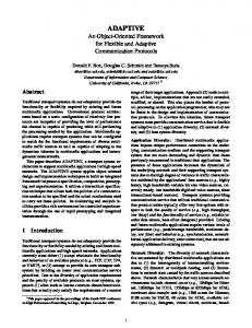
which corresponds to a ratio dB. Additive noises are zero mean, white, Gaussian and mutually independent. For and each pair of randomly generated channels, are estimated according to (30), (31) with a forgetting factor , and then averaged over 100 trials. Step sizes used in simulations are 0.003 for both equalizers. The number of taps for the SOC-MI-DFE, is 20 (14, 1, 5) in each transverse filter and 4 in each recursive filter, while, it is 25 (12, 1, 12) in each transverse filter for the blind MI-LE. The initial coeffi, cients vectors are: and . The main conclusion to be drawn from simulations is that the SOC-MI-DFE, when held in its starting-up mode (Fig. 9), exhibits a faster convergence and a weaker residual DDMSE than the MI-LE (Fig. 10). It is also interesting to note the striking similarity between the DDMSE and the estimated Godard error. As a result, the Godard criterion can also be used for selecting the relevant running mode, provided a slightly different threshold is used. Fig. 11 compares the performance of the SOC-MI-DFE and the (single input) SOC-SI-DFE [8] using the 100 discrete chanpreviously generated, with snr dB. It clearly nels appears that the two-dimensional equalizer largely outperforms its one-dimensional counterpart, in terms of both speed of convergence and DDMSE. In addition, the SOC-MI-DFE clearly improves the performance of the blind MI-LE (see Fig. 9). In order to show the superiority of this novel approach, the mean time required to reach the appropriate switching threshold

V. UWA COMMUNICATIONS SIGNALS The SOC-MI-DFE has been successfully tested on real signals originating from experimentation carried out near Brest (France) by the French “Groupe d’Etudes Sous-Marines Atlantique” (GESMA) with the main purpose of testing the efficiency of high data bit rate acoustic links. The number of sensors used in this experiment was 48, the modulation scheme QPSK, the bit rate 16.67 kbps and the carrier frequency 62 kHz. The estimated impulse response on a given channel is depicted in Fig. 12. It exhibits very strong intersymbol interference, with a delay spread of 55 symbol durations . Furthermore, at the very beginning of the file, the channel proves to be fast time-varying, which explains the difficulty encountered by the conventional trained DFE. In what follows, the novel blind SOC-MI-DFE is compared to the conventional MI-DFE which is first trained by a sequence of 1000 known data symbols and then decision-directed. The number of taps is 15 for each forward filter and 60 for the backward filter. Timing recovery is carried out with the Gardner algorithm [17]. In Fig. 13, one can observe that the one-dimensional trained DFE does not work since it has converged toward . a bad solution where the decision-directed (not true) MSE The situation is essentially the same when using two sensors. Needless to say that, despite a very small estimated DDMSE, the trained DFE output is completely irrelevant since it has converged toward a pathological fixed point. The reason is that the channel proves to be quite severe (see Fig. 12), at the very beginning of the file. The main drawback of the trained DFE is once again highlighted. Since the equalizer has not converged during the training sequence, it evolves toward a pathological stable

LABAT AND LAOT: BLIND ADAPTIVE MI-DFE WITH A SELF-OPTIMIZED CONFIGURATION

653

TABLE I COMPARISON BETWEEN

THE

MI-LE,

THE

SOC-MI-DFE

AND THE SOC-SI-DFE IN TERMS OF TO REACH THE THRESHOLD J

ASYMPTOTIC DDMSE

AND

TIME REQUIRED

very severe and, in such conditions, the use of a conventional DFE requires periodical training sequences in order to avoid catastrophic error propagation phenomena. Despite these harsh conditions, the novel “blind” equalizer proves to be very efficient. VI. CONCLUSION

Fig. 12. Time-varying impulse response (modulus) of the UWA channel for a period of 5 s.

This paper brings an original answer to the question about how to “blindly” drive the filter coefficients of the MI-DFE in order to approach the MMSE-DFE solution. In terms of robustness, steady state MSE and convergence speed, the novel (blind) SOC-MI-DFE [18] outperforms the conventional blind MI-LE [16] that represents the state of the art among the blind adaptive equalizers of reasonable complexity. Even though it has been investigated in the special case of two receivers, the underlying principle can be easily extended to the case of more than two receivers, including fractionally-spaced equalizers. Furthermore, the good behavior of the new equalizer has been verified through UWA communications signals, in very severe environments. To conclude, not only is this novel blind approach of real interest from a theoretical point of view but its very high speed of convergence also renders it competitive in various standard applications, even in the case of burst mode transmission systems. In the UWA communications field, the SOC- MI-DFE is going to be implemented on a DSP: the target is typically to reach a few tens of kbps in the 0–2 km (shallow water) range. APPENDIX

Fig. 13. Conventional trained MI-DFE vs. blind SOC-MI-DFE in terms of estimated MSE (dB).

fixed point: the equalizer is then totally lost and needs retraining. On the other hand, a 4 sensor conventional trained MI-DFE does succeed and exhibits quite good behavior in the process of mitigating ISI. At the same time, the blind SOC-MI-DFE exhibits an ideal behavior, even in the case of 1 or 2 sensors. The following plots of Fig. 13 depict the evolution of the estimated MSE. One can also notice that, in the cases of both blind and trained (4 sensors) MI-DFE, the speed of convergence is roughly the same. The spikes which appear on the DDMSE originate from the boat depth sounder, the frequency of which was in the signal bandwidth, with a period of 1.2 s between each burst, which symbol durations . In practice, this jammer is represents

According to the orthogonality principle, the optimal MMSE solution can be obtained by developing the following system:

and

(A-1)

Defining the correlation functions for for for

(A-2) (A-3) (A-4)

654

IEEE TRANSACTIONS ON COMMUNICATIONS, VOL. 49, NO. 4, APRIL 2001

(A-7)

and with

denoting the convolution operator, this becomes:

for all

(A-5)

Using the bilateral -transform, and after some simple arrangements:

(A-6)

and is unique and given by (A-7), The solution for shown at the top of the page. It is also interesting to note that in , solutions the noiseless case, i.e., if and obey the following underdetermined system: (A-8) ACKNOWLEDGMENT The authors would like to thank the reviewers for their helpful and nice suggestions and comments. Furthermore they would also thank all those who contributed to improve the paper readability, namely J. Ormrod and I. Simpson from ENST Bretagne, and all those who helped them by their encouragement and fruitful discussions. REFERENCES [1] J. G. Proakis, Digital Communications, 2nd ed: McGraw-Hill Company, 1989. [2] P. Balaban and J. Salz, “Optimum diversity combining and equalization in digital data transmission with applications to cellular mobile radio—Part I and II,” IEEE Trans. Commun., vol. 40, pp. 885–907, May 1992. [3] L. Tong, G. Xu, and T. Kailath, “A new approach to blind identification and equalization based of multipath channels,” in Proc. 25th Asilomar Conf., Pacific Grove, CA, 1991, pp. 856–860. [4] , “Fast blind equalization via antenna arrays,” in Proc. ICASSP, vol. 4, 1993, pp. 272–275. [5] L. Tong, G. Xu, B. Hassibi, and T. Kailath, “Blind identification and equalization based of multipath channels: A frequency domain approach,” IEEE Trans. on IT., March 1994. [6] E. Moulines, P. Duhamel, J. F. Cardoso, and S. Mayrargue, “Subspace methods for the blind identification of multichannel FIR filters,” IEEE Trans. Signal Processing, vol. 43, pp. 516–525, Feb. 1995. [7] J. Labat, C. Laot, and O. Macchi, “Dispositif d’égalisation adaptatif pour systèmes de communications numériques,” French Patent 9 510 832, Sept. 15, 1995.

[8] J. Labat, O. Macchi, and C. Laot, “Adaptive decision feedback equalization: Can you skip the training period?,” IEEE Trans. Commun., vol. 46, pp. 921–930, July 1998. [9] C. A. Belfiore and J. H. Park, “Decision feedback equalization,” Proc. IEEE, vol. 67, pp. 1143–1156, Aug. 1979. [10] D. N. Godard, “Self-recovering equalization and carrier tracking in two dimensional data communication system,” IEEE Trans. Commun., vol. COM-28, pp. 1867–1875, 1980. [11] D. D. Falconer, “Jointly adaptive equalization and carrier recovery in two-dimensional data communication systems,” Bell Syst. Tech. J., vol. 55, pp. 317–334, March 1976. [12] B. Picinbono, Signaux Aléatoires: Base du Traitement Statistique du Signal. Tome 3: Dunod. [13] O. Macchi, Adaptive Processing. The LMS Approach with Applications in Transmission. New York: Wiley, 1995. [14] O. Shalvi and E. Weinstein, “New criteria for blind deconvolution of nonminimum phase systems (channels),” IEEE Trans. Inform. Theory, vol. 36, pp. 312–321, Mar. 1990. [15] V. Shtrom and H. Fan, “New class of zero-forcing cost functions in blind equalization,” IEEE Trans. Signal Processing, vol. 46, pp. 2674–2683, Oct. 1998. [16] S. Mayrargue, “A blind spatio-temporal equalizer for a radio-mobile channel using the constant modulus algorithm (CMA),” in Proc. ICASSP94, pp. 317–320. [17] F. M. Gardner, “A BPSK/QPSK timing-error detector for sampled recivers,” IEEE Trans. Commun., vol. COM-34, pp. 423–429, May 1986. [18] J. Labat and C. Laot, “Dispositif d’égalisation adaptative pour récepteurs de communications numériques multivoies,” French Patent 9 914 844, November 1999. , “Egalisation autodidacte adaptative: Application aux systèmes [19] d’accès à répartition dans le temps,” in 17th GRETSI Symp., vol. 4, Vannes, France, Sept. 1999, pp. 1081–1084.

Joel Labat was born in Dakar, Sénégal, in 1951. He received the Eng. degree from the Conservatoire National des Arts et Métiers (CNAM), Brest, France, in 1989, and the Ph.D. degree from the University of Bretagne Occidentale (UBO), Brest, France, in 1994. He is presently with the Ecole Nationale Supérieure des Télécommunications de Bretagne (ENST Bretagne), Brest, France, as Directeur d’études. His research interests include digital communications over multipath channels and related problems such as blind equalization, synchronization and signal processing. His favorite fields of investigations are both underwater acoustic communications and wireless communications.

Christophe Laot was born in Brest, France, on March 12, 1967. He received the Eng. degree from the Ecole Francaise d’Electronique et d’Informatique (EFREI), Paris, France, in 1991 and the Ph.D. degree from the University of Rennes 1, Rennes, France, in 1997. He is currently with the Digital Communications Team, Ecole Nationale Supérieure des Télécommunications de Bretagne (ENST Bretagne), Brest, France. His professional interests include equalization, channel coding, turbo-equalization and interference suppression in CDMA systems.