convergence speed of a blind algorithm is to apply a sequence of gradually ..... For the baud-rate feed forward linear equalizer adopting the stop-and-go ...
1
ADAPTIVE BLIND EQUALIZERS WITH AUTOMATICALLY CONTROLLED PARAMETERS TERM 001
EE 511 DETECTION & ESTIMATION
KAMRAN ARSHAD ID # 210261
SUBMITTED TO Dr. Asrar-ul Haq Sheikh
DEPARTRMENT OF ELECTRICAL ENGINEERING
KING FAHD UNIVERSITY OF PETROLEUM AND MINERALS
2
ABSTRACT
Signals when pass through a channel undergo various forms of distortion, most common of which is Inter-symbol-interference, so called ISI. Inter-symbol interference induced errors can cause the receiver to misinterpret the received samples. Equalizers are important parts of receivers, which minimizes the linear distortion produced by the channel. If channel characteristics are known a priori, then optimum setting for equalizers can be computed. But in practical systems the channel characteristics are not known a priori, so adaptive equalizers are used. Adaptive equalizers adapt or change the value of its taps as time progresses. There are two main types of adaptive equalizers, trained equalizers and blind equalizers. In trained equalizers there is a pseudo-random pattern of bits called training sequence known both to receiver and transmitter. But equalizers for which such a initial training period can be avoided are called BLIND EQUALIZERS. Blind equalizer as opposed to data trained equalizer, is able to compensate amplitude and delay distortion of a communication channel using only channel output sample and knowledge of basic statistical properties of the data symbol. Among some algorithms of blind equalizers like CMA, Stop and Go, GSA, SGA, SRCA etc., Stop and Go is one of the most important algorithms. Unfortunately all blind equalizers converge very slowly. So there is a proposed method for automatic control of step size and filter length for a blind equalizer which is driven by stop and go directed algorithm. This idea was presented by Krzysztof Wesolowski in his paper “Adaptive Blind Equalizers With Automatically Controlled Parameters”. This proposed method for varying the step size results substantial shortening of the convergence time.
3
1. INTRODUCTION: A Blind Equalizer, as opposed to a data-trained equalizer, is able to compensate amplitude and delay distortions of a communication channel using only the channel output samples and the knowledge of the basic statistical properties of the data symbols. Among a few adaptation algorithms developed so far, the stop and go algorithm [1] is one of the most important. Unfortunately, all realizable, gradients – type blind algorithms converge very slowly. One of the simplest ways to increase the convergence speed of a blind algorithm is to apply a sequence of gradually decreasing adaptation steps which better fit the current state of the convergence process than the constant step size [2]. Recently usefulness of controlling the length of transversal equalizer resulting in increasing of the convergence speed has been discovered [3] and analyzed [4]. The same idea was also briefly mentioned in [5], however, without any explanation.
2. ADAPTIVE EQUALIZATION: In digital communications, a considerable effort has been devoted to the study of data transmission system that utilizes the available channel bandwidth efficiently. The objective here is to design a system that accommodates highest possible rate of data transmission, subject to a specified reliability that is usually measured in terms of the error rate or average probability of symbol error. The transmission of digital data through a linear communication channel is limited by two factors. 1- Inter Symbol Interference. (ISI) 2- Thermal noise ISI is caused by dispersion in the transmit filter, the transmission medium, and receive filter. The receiver at its front end generates thermal noise. For bandwidth-limited channels (e.g., voice-grade telephone channels), we usually find that inter symbol interference is the chief determining factor in the design of high data rate Transmission systems.
4
Input binary data
Pulse generator
Transmit Filter
Recieved Filter
+
Medium
NOISE
Transmitter
Decision Device
Output binary data
Receiver
Block diagram in Figure shows the equivalent base band model of binary pulseamplitude modulation (PAM) system. The signal applied to the input of the transmitter part of the system consists of binary data sequence, in which each symbol consists of 1 or 0. This sequence is applied to the pulse generator, the output of which is filtered first in the transmitter, then by the medium, and finally in the receiver. Let u(k) denote the sampled output of the receiver filter in the block diagram; the sampling is performed in synchronism with the pulse generator in the transmitter. The output is compared with a threshold by means of a decision device. If the threshold is exceeded, the receiver makes a decision in favor of symbol 1. Otherwise it decides in favor of symbol 0 Let a k be a scaling factor defined by, a k = { +1 if the input consists of symbol 1
-1 if the input consists of symbol 0 } Then in the absence of thermal noise, we may express
u (k ) =
∑a
n
p(k − n )
n
= a k p(0) +
∑ a p(k − n ) n
(n ≠ 0)
n
where p(n ) is the sampled version of the impulse response of the cascaded connection of the transmitter filter, the transmission medium, and the receiver filter. The first term of the right hand side of equation (1) defines the desired symbol, whereas the remaining series represents the inter symbol interference caused by the channel. The inter symbol interference, if left unchecked, can result erroneous
5 decisions when the sampled signal at the channel output is compared with some pre assigned threshold by means of decision device. To overcome the ISI, control of the time-sampled function p(n ) is required. In principle, if the characteristics of the transmission medium are known precisely, then it is virtually always possible to design a pair of transmit and receive filters that will make the effect of inter-symbol-interference (at sampling times) arbitrary small. But the use of a fixed pair of transmit and receive filters, designed on the basis of average channel characteristics, may not adequately reduce the ISI. This suggests the need for an “Adaptive Equalizer” that provides precise control over the time response of the channel. Among the basic philosophies for equalization of data transmission systems are pre equalization at the transmitter and pre equalization at the receiver. Since the former technique require the use of feed` back path, we will only consider equalization at the receiver, where the adaptive equalizer is placed after the receive filter. In theory, the effect of ISI may be made arbitrary small by making the number of adjustable coefficients (tap weights) in the adaptive equalizer infinitely large. An adaptive filtering algorithm requires the knowledge of the “desired” response so as to form the error signal needed for adaptive process to function. In theory, the transmitted sequence (originating at the transmitter output) is the “desired” response for the adaptive equalization. In practice, however, with the adaptive equalizer located at the receiver, the equalizer is physically separated from the origin of its ideal desired response. One method to generate the desired response locally in the receiver is the use of training sequence, in which a replica of the desired response is stored in the receiver. Naturally the generator of this stored reference has to be electronically synchronized with the known transmitted sequence. With a known training sequence, the adaptive filtering
algorithm
used
to
adjust
the
equalizer
coefficients
corresponds
6 mathematically to searching for the unique minimum of quadratic error-performance surface. Second method is decision directed method, in which, a good facsimile of the transmitted sequence is being produced at the output of the decision device in the receiver. Accordingly, if this output were the correct transmitted sequence, it may be used as the “desired” response for the purpose of Adaptive Equalization.
Channel Output
ak
Receiver Output
RECIEVER
Channel Input
Channel
Equalizer
Decision Device
Channel Equalization in a Data Communication System
3. BLIND EQUALIZATION: Blind Equalization perform channel equalization without the aid of a training sequence. The term blind is used because the equalizer performs the equalization blindly on the data without a reference signal. Instead the blind equalizer relies on the knowledge of signal’s structure and its statistics to perform the equalization. The major advantage of blind equalizers is that there is no training sequence at the start up, hence no bandwidth is wasted by its transmission. The major drawback is that the equalizer will typically take a longer to converge as compared to a trained equalizer. The need for blind equalizers in the field of data communications is greatly discussed by Godard[2], in the context of multipoint networks. Blind joint equalization and carrier recovery may also find application in digital radio link over multipath fading
aˆ k
7 channels. Moreover, in highly non stationary environments like digital mobile communications, it is impractical to use training sequences. Furthermore, application of blind equalization is also important, in other areas, such as geographical signal processing.
3.1 QAM SIGNALS Suppose in a typical communication system, if the data rate is 32kb/s, and the signaling rate is 16kb/s, than every bit transmitted must carry two bits of information. This mean that we must have four points on the constellation, and clearly this can be done in many ways. Figure shows some four points constellation.
00 10
00
10
01
01
(a)
11
11
(b)
00
01
10
11
00
01
10 11 (c)
(d)
8
The two bits of information associated with each constellation point are marked on the figure. In part (a) and (b) so called quadrature modulation has been used as the points can only be uniquely described using two orthogonal coordinate axes, each passing through the origin. The orthogonal coordinate axes have a phase rotation of 90 degrees with respect to each other, and hence they have so called quadrature relationship. The pair of coordinate axes can be associated with a pair of quadrature carriers, normally have a sine and cosine waves, which can be independently modulated and than transmitted within the same frequency band. Due to their orthogonality
they can be separated by the receiver. This implies that whatever
symbol is chosen on one axis it will have no effect on the demodulated on the y axis. Data can therefore be independently transmitted via these two quadrature or orthogonal channels without any increase in error rate. For the constellation of part (a) and (b) we have a constant amplitude signal, but the carrier phase values at the beginning of each symbol period in figure (b) would be either 45 deg, 135 deg, 225 deg or 315 deg. These are two magnitude values and two phase values for the constellations in figure (c) and (d). In general, grouping n bits into one signaling symbol yields 2n constellation points, which are often referred to as phasors, or complex vectors.
9
3.2 BLIND EQUALIZATION IN "QAM" DATA TRANSMISSION SYSTEMS A typical QAM (Quadrature amplitude modulated) data transmission system consists of transmitter, a channel, and a receiver, where the unknown channel represents all the interconnections between the transmitter and the receiver. The transmitter generates a zero mean, independent input data sequence { a k }, each element of which comes from a finite alphabet A of the QAM symbols (or constellation). The data sequence { a k } is sent through the channel whose output { x k } is the receiver input. The function of the receiver is to restore the original data { a k } from the observation { x k } by outputting a sequence of estimate { a k }. Assume the channel is linear, causal, and (BIBO) stable with transfer function
H (q −1 ). Its input-output relation can be written as H (q −1 ) × a k =
∑
∞
i =0
hi × a k −i ,
a k −i ∈ A ⊂ ∆ , hi ∈ ∆
such that more than one non-zero element exists in Where { hi } is the impulse response of the channel. When the channel is ideal with no ISI such that only one nonzero element exists in the sequence { hi }, then the channel output becomes
x k = hv × a k −v ,
hv ≠ 0,
v ∈ Ζ+
Which is simply the scaled version of the input with finite delay v . In this ideal case, the original sequence can be recovered by removing the constant scaling factor through an appropriate memory less nonlinear decision device. The difficulty arises when the channel is imperfect such that more than one non-zero element in the channel impulse response. In this case an undesirable ISI is introduced at the channel output from which a simple memory less decision device might not be able to recover the original data sequence.
( )
A linear channel equalizer is a linear filter G q −1 applied to the channel output to eliminate its ISI by essentially canceling the channel dynamics. All the ISI is removed if
10
G (q −1 ) H (q −1 ) = cq − v , 0 ≠ c ∈ ∆ , v ∈ Ζ + such that the equalizer output becomes z k = ca k −v . The desired response can be rewritten as
G (q −1 ) = cq − v [ H (q −1 ) ] -1, Which means that the equalizer attempts to achieve the inverse of the channel transfer function with a possible gain difference and/or a constant time delay. In blind equalization, the original sequence is unknown to the receiver except for its probabilistic or statistical properties over the known alphabet A . Based on the second-order statistics of the input and output signal of the channel, the spectral magnitude of the channel can be determined and so that of the channel inverse. Thus if the channel is known to be of minimum or maximum phase, only second order
( )
statistics need to be used to identify H q −1 , with which one can construct, respectively, a truncated causal or an anticausal inverse of the channel using an FIR Equalizer. Unfortunately, communication channels usually have mixed phase. Hence, the blind equalization problem for general channels cannot be solved through schemes that only use second order statistics. If the input sequence is gaussian, so is the output. Therefore, only second order statistics are useful if the input is gaussian which means that blind equalization is unattainable for gaussian input with mixed-phase channels. In summary, the following facts about the blind equalization are generally noted.
•
A mixed-phase linear dynamical channel is identifiable from its output (and knowledge of the distribution of its input) only when the input is not gaussian.
•
Second order statistics alone are generally insufficient for blind equalization.
•
No channel transfer function zeros are allowed on the unit circle, since spectral nulls require a linear equalizer with infinite gain to compensate.
•
An exact causal inverse of a nonminimum-phase channel is unstable. However an anticausal representation can be truncated and delayed with a finite delay v to enable a causal equalizer to approximate the desired response.
11
•
Most practical QAM systems employ a constellation, which has symmetrical properties. If the input data is independent and uniformly distributed over constellation, a kπ / 2 phase rotation does not cause any statistical changes in the channel output. Thus the data recovered from blind equalization will be subjected to a phase ambiguity of kπ / 2 , and the best possible result would be G (q −1 ) H (q −1 ) =
e kπ / 2 q − v , k ∈ {0,1,2,3}
Thus remaining phase ambiguity can be resolved through differential encoding.
3.3 BLIND EQUALIZATION ALGORITHMS Sato was the first who introduced the idea of blind equalization for multilevel pulse amplitude modulation, and after it Godard combined Sato idea with a Decision Directed algorithm and obtain a new blind equalization scheme for QAM data transmission. Sato proposed algorithm which was designed only for real valued signal and PAM. However, its complex valued extension is straightforward which was derived by Godard.
I) Sato Algorithm
Sato algorithm dedicated to real valued signal z(n), which uses the following cost function: J(n) = E [ ( z(n) - γ )2 ] Where γ is the sato’s coefficient and z(n) is the equalizer output. Sato’s coefficient update equation is given as: C(n+1) = C(n) – µ. y∗(n). εsato(n) Where εsato(n) is the Sato’s error defined as: εsato(n) = z(n) – γ csgn(z(n)) so taps of equalizer are updated according to the equation defined above. As it can be seen from above equation, this algorithm uses only the sign of equalized output values z(n) in order to update equalizer coefficients C(n). Setting the value of γ in above
12 equation is very important, since it actually directs the signal z(n) to the point of its convergence that is to the original constellation points. The optimum value of γ set by Sato in order to achieve minimum MSE is given by: γ = E [ a(n) 2 ] / E [ abs( a(n) ) ] which is only for real valued signals, where a(n) is the signal to be transmitted. A typical equalization scheme looks like: e(n)
a(n)
y(n)
CHANNEL hi
+
EQUALIZER Ci
z(n)
DECEISIO N DEVICE
dec(a(n))
EQUALIZED COMMUNICATION SYSTEM
II) Constant Modulus Algorithm (CMA)
Godard algorithm which he developed for complex valued signal is the most popular scheme for blind equalization of QAM signals. The CMA attempts to minimize the constant modulus cost function JCM. CMA adjust the taps of equalizer in an attempt to minimize the difference between samples squared magnitude and Godard dispersion constant R2, which depends only on input data symbols { a k }. So value of JCM depends on difference between squared magnitude of received samples z(n) and the Godard dispersion constant γ. JCM = E [ ( abs( z(n) )2 – R2 )2 ] Where z(n) is the equalizer output at time n. The equalizer coefficient update equation in CMA uses a gradient descent to minimize JCM. The equation is given by Godard as, C(n+1) = C(n) - µ .y∗(n). z(n). [ (abs( z(n) )2 – R2 ] Where in order to find out the value of R2, Godard uses the exactly same method as used by Sato, to obtain the value of R2, R2 = E [ a(n) 4] / E [ abs( a(n) )2 ]
13 III) Modified Constant Modulus Algorithm (CMA)
Another modified version of Godard’s CMA was proposed by Wesolowsky, employing a cost function, which relies on both the real and imaginary parts of the equalized signal z(n). J(n) = E [ (abs( Re{z(n)} )2 – R2,R )2 + (abs( Im{z(n)} )2 – R2,I )2 ] The idea behind this cost function, as compared to the CMA cost function, is that both the real and imaginary parts of the signal are forced to a constant value and, therefore, the random phase ambiguity of CMA now becomes only 90 degrees. This is meaningful in a pure phase modulation, in which case the CMA may converge to an arbitrary phase shifted solution. For QAM though, the 90 degree symmetry of the constellation make it possible for both algorithm to converge to a 90 degree phase shifted solution. Now here the coefficient update equation is: C(n+1) = C(n) - λ y(n). [Re(z(n)).((Re(z(n))2 –R2,R) + j Im(z(n)).((Im(z(n))2 –R2,I)]. The values of R2,R and R2,I can be calculated by exactly the same method as used by Sato and Godard in their algorithms. R2,R = E [Re( a(n)) 4] / E [ Re( a(n) )2 ] R2,I = E [Im( a(n) ) 4] / E [ Im( a(n) )2 ] Wesolowsky also showed that the MCMA exhibits slightly faster convergence than the classical CMA, in particular for medium distortion channels. He also showed that his algorithm offers slightly better steady state performance.
4 STOP AND GO" DECISION DIRECTED ALGORITHM FOR BLIND EQUALIZATION `In my term paper, I am using "STOP AND GO" decision directed algorithm, proposed by GIORGIO PICCHI and GIANCARLO PRATI, which is not based on the knowledge of complex output error en . The term “STOP AND GO” indicates that every time, tap coefficients are not adapted, instead the reliability of error is checked and then the algorithm decides either the tap coefficients should be adapted or not. It is worth exploring the possibility of retaining the advantages of simplicity and smoothness of the decision directed algorithm while attempting to substantially improve its blind convergence capabilities. The basic idea
14 in the paper of picchi prati was that this possibility could be achieved by stopping adaptation when the reliability (in a probabilistic sense) of the self-decided output error is not high enough. More precisely an easy to generate “binary-valued flag” tells the equalizer whether the output error on the current decision may be reliably used in the standard Decision Directed algorithm. If not, adaptation is stopped for that iteration. The stop and go operation made of the standard DD algorithm is an attractive solution of the problem of blind joint equalization and carrier recovery. As a matter of fact, this algorithm has been successfully implemented and tested in a new commercial 64QAM digital radio system. In this algorithm, two SATO-like errors ~ en , R = y n , R − (sgn y n , R )β n ~ en , I = y n , I − (sgn y n , I )β n are generated. where y n , R and y n , I are the real and imaginary components of the output of the equalizer. β n being a suitable real value possibly changing with n , and used to determine on which intervals of y R and y I axes, the error on the decided symbol may be used for adaptation. More specifically, the DD Algorithm now uses the following binary-valued flags.
fn , R = { 1 0 f n , I = {1 0
∧
if sgn en , R = sgn e~n , R ∧
if sgn e n , R ≠ sgn e~n , R if
∧
sgn en , I = sgn e~n , I ∧
en , I if sgn e n , I ≠ sgn ~
∧
where en is the estimated error, determined by the relation. ∧
en = ( y n , R − dˆ n , R ) + j ( y n , I − dˆ n , I )
15 Note that dˆ n is the decision made in each interval that our output of equalizer y n is nearest to which one signal in the given 64-QAM-signal constellation. ∧
When the event { sgn en , R = sgn e~n , R } occurs and the choice of β n is proper, the conditional error probability,
Pn / go = P{no _ error | go} = P{sgn eˆn , R = sgn en , R | sgn eˆn , R = sgn e~n , R }
= P{sgn eˆn , I = sgn en , I | sgn eˆn , I = sgn e~n , I } ∧
is sufficiently high, and sgn en , R may be confidently used in the DD Algorithm. The two flags f n , R and f n , I therefore restrict operation of algorithm to a region of higher reliability. It can be shown that by a direct measure of some performance parameters, a proper choice of β n can be made, favorable on the average. Therefore ∧
∧
β n is used as a reference point to identify regions on each axis where en , R and en , I may be used more confidently. The conditional error probability p n / go and its complement q n / go = P{error | go} = 1 − p n / go corresponds in a sense to p n and q n . The performance related to the probabilities is better than all other algorithms. p n / go = P{no _ error | go} = P{sgn eˆn , R = sgn en , R, f n , R = 1} = P{sgn eˆn , R = sgn en , R, . sgn eˆn , R = sgn ~ en , R} = (1 − p sc ) p n q n / go = P{error | go} = P{sgn eˆn , R ≠ sgn en , R, f n , R = 1} = P{sgn eˆn , R ≠ sgn en , R,
. sgn eˆn , R = sgn e~n , R} = (1 − p se )q n
16 A proper choice of β n causes q n / go to be sufficiently smaller than q n / DD , that is, adaptation stops with probability p se when a sign error occurs for a component of eˆn . This makes the Decision Directed Algorithm converge. For the baud-rate feed forward linear equalizer adopting the stop-and-go algorithm, the filter coefficient update equation is given as c(n + 1) = c(n) + e SG (n) *
where α is the adaptation step size, c T (n) = [c 0 (n), c1 (n), c 2 (n),............c N −1 (n)] is the coefficient vector, x T (n) = [ x(n), x(n − 1),...., x(n − N + 1)] is the input vector, e SG (n) , produced by processing the equalizer output y (n) , is the error signal at time n , and N is the number of equalizer tap coefficients.
The stop and go Algorithm uses the Decision Directed algorithm (DD) error signal and allows coefficient updates only when the DD error signal is considered to be reliable. The DD error signal is given by eˆ(n) = y (n) − dˆ (n)
where dˆ (n) is the decision made on the data symbol a(n − D) from y (n) and D is the overall propagation delay of the channel and the equalizer. A method of judging the reliability of the DD error signal is to see whether the sign of the DD error coincides with a sato-like error ~ e (n) = y (n) − β SG [sgn( yR(n)) + j sgn( yI (n))] where R and I denotes the Real and Imaginary components of the Equalizer output y (n)
and β SG is a suitable real value chosen depending upon the data constellation.
Hence the real and imaginary parts of the error signal for the stop and go algorithm are given as follows eγSG ( n) = f γ (n)eˆγ ( n)
,
where
for γ = I , R (i.e. indicating Real and Imaginary parts) f γ ( n) = {
0,
1, if sgn(~eγ (n)) = sgn(eˆγ (n))
otherwise
γ = I, R
17
5. THE CONTROLLED LENGTH BLIND EQUALIZER It has been proven [6] that the step size of the regular gradient algorithm applied to the reference data-trained equalizer is inversely proportional to the equalizer length. The longer the equalizer, the smaller is the step size required to ensure the stability of the algorithm, which in turn lengthens the convergence time. The shorter the equalizer converges faster but the residual mean square error is higher. One can also observe that after convergence, the main proportion of the energy of the equalizer’s coefficients is usually concentrated around the main tap. Thus, through the adjustment of the few coefficients in the middle of the equalizer, a rough equalization is achieved. It [3] has been shown that such a simple idea leads to a large reduction of the convergence time especially when the stop and go blind algorithm is applied. Unfortunately, the optimum moment of switching depends on particular channel characteristics. It would also be desirable if the equalizer could change its length and quickly recover its coefficients when the channel suddenly changes. Thus, the automatic switching of the equalizer length and the related step size is a very desirable feature even at the cost of some convergence slowdown as compared with the case when the step size and the moment of changing is best matched to a particular channel.
6. AUTOMATIC CONTROL OF EQUALIZER PARAMETERS (USING STOP-AND-GO ALGORITHM)
An ad hoc method of controlling the equalizer’s length and its step size is proposed below for the stop and go blind algorithm, which is particularly well suited for our purpose. Below are the equations of the algorithm
y (n) = ∑i = − N c i (n).x(n − i ) N
eˆ(n) = y (n) − dˆ (n)
18 where dˆ (n) = dec( y (n))
c i (n + 1) = c i (n) − γ n [ f nR Re(eˆ(n)) + j. f nI Im(eˆ(n))].x * (n − i ) for i = − N ,........... + N where f nR and f nI are the On and Off coefficients (described in the paper of Picchi and Prati) .
c i (n)
are the equalizer’s coefficients and x(n − i) is the input signal
contained in the tapped delay line of the equalizer on the ith position . Function dˆ ( n) = dec( y (n))
described the operation of a decision device, which generates the
output as the signal constellation point closest in the Euclidean sense to the signal y (n) .
One can easily note that the magnitude of the output error eˆ(n) can be
considered as a measure of how far the coefficients are located from their optimum. One can appropriately select the area around each signal point on the signal constellation plane. If the subsequent equalizer output signals y (n) fall into these areas, one can expect that rough equalization have already been achieved. For a square QAM signal constellation when Re(d n ) and Im(d n ) belong {±1,±3,±5,..............,± (2 m − 1)}
to
the
set
and (2 m − 1) is the largest in phase or quadrature data
symbol component, the area of the i − th constellation point can be defined as follows. y ( n) ∈ Di
if and only if | Re( y (n)) − Re(d i ) |≤ ∆
and
| Im( y (n)) − Im(d i ) |≤ ∆
(Condition 1)
where ∆ is properly selected constant. Because the distance of the data symbol Inphase or Quadrature component to the nearest threshold is equal to one. Obviously
∆ N I
, γ1 < γ 2
and 2 N I + 1 is the full length of the equalizer. The same
procedure can be applied to control the step size only. Thus N 1 = N 2 = N . No general theory on the selection of the step size for a blind equalizer algorithm exists so researchers usually resort to the simulation experiments. Generally the step size
γ 2 should ensure stable operation of the short or full-length equalizer at the beginning of the convergence process and γ 1 should be selected with respect to the low excess error in the steady state. The step size γ 2 is kept usually much smaller than that derived by Ungerboeck [6] by the relation
γ 0 = 1 /((2 N1 + 1) E[| x n | 2 ]), where E[| x n | 2 is the mean input signal power. The above equation gives the optimum initial step size for the gradient adjustment of the data trained equalizer. Because the event y (n) ∈ Di has a probabilistic character turning the adaptation of the shorter or longer equalizer on and off and / or higher or lower step size on and off, will not be smooth. A single event y(n) ∈ Di can already switch the adaptation of the longer equalizer on, although the equalizer can be far away from rough equalization of the channel. To protect it accidental turning the adaptation of the longer equalizer on, the algorithm can monitor a few recent values of the output error eˆ(n) . A very simple monitoring method is proposed which can be implemented.
7. SIMULATION RESULTS The operation of a blind transversal equalizer with automatically controlled length and step size of the stop and go algorithm was verified using a simulation experiment. The channel reported by G. Picchi and G. Prati in [1] was applied in our simulations. Transmissions using 64-QAM modulations Re(d n ), Im(d n ) ∈ {±1 , ± 3 , ± 5 , ± 7}
21 was simulated. The additive gaussian noise samples were added on the output of the channel. SNR = 30 dB , E[| xn |2 ] = 42,
Figure 1 (CONSTANT STEP SIZE AND LENGTH OF EQUALIZER)
Shows the Equalized 64-Qam Constellation and curve for Mean Square Error versus iteration number for the constant length and step size of
γ n = 5 × 10 −4 . Constant
length means that all the tap coefficients are adapted . For this case length of the equalizer is taken to be 15.
Constant Step Size 15
10
M ean Square E rror
5
0
-5
-10 0
1000
2000
3000
4000
5000 6000 Number Of Iterations
7000
8000
9000
10000
22
Figure 2 (VARIABLE STEP SIZE AND CONSTANT LENGTH OF EQUALIZER)
Shows the algorithm with the variable step size i.e. γ n = 5 × 10 −4 when condition (1) | Re( y ( n)) − Re(d i ) |≤ ∆
and
| Im( y (n)) − Im(d i ) |≤ ∆
(Condition 1)
with ∆ = .75 is fulfilled. γ n = 1 × 10 −3
otherwise.
Variable Step Size 15
M ean S quare E rror
10
5
0
-5
-10 0
1000 2000 3000 4000 5000 6000 7000 8000 9000 10000 Number Of Iterations
23 Figure 3 (CONSTANT STEP SIZE AND VARIABLE LENGTH OF EQUALIZER)
Shows the algorithm for the equalizer with automatically controlled length when condition (1) | Re( y (n)) − Re(d i ) |≤ ∆
and
| Im( y (n)) − Im(d i ) |≤ ∆
____
(1)
with ∆ = .75 is fulfilled. If the above condition is fulfilled, then all the tap coefficients are adapted; otherwise only five tap coefficients around the main one are adapted. Variable LENGTHANDStepSize 12
10
8
6
M ean S quare E rror
4
2
0
-2
-4
-6
-8 0
1000
2000
3000
4000
5000 6000 Number Of Iterations
7000
8000
9000
10000
24
AUTOMATIC LENGTH CONTROL
It is to be clear that variable length equalizer means that the number of tap coefficients, which are adapted, varies. Switching between adaptations of all taps coefficients or a part of them is performed. From figure 3, the influence of the automatic length control on the convergence speed of the constant step size equalizer was investigated. The full length of the equalizer is taken to be 15. All the equalizers are adapted with the same step size of γ n = 5 × 10 −4 , which ensures the same residual mean square error. For the short equalizer only five coefficients around the main tap were adapted through the whole length of the delay line and all the coefficients were used to generate the output signal. Let us note that at the beginning, when the short equalizer starts to adapt its coefficients, those at both ends of the delay line do not take part in generation of the output signal because they are equal to zero. However, if during the adaptation process, the full-length equalizer is subsequently switched on and off, all the coefficients become different from zero and in consequence all of them are used in the calculation of the output signal although, temporarily, only those in the middle of the delay line are further adjusted.
25
Figure 4 (VARIABLE STEP SIZE AND VARIABLE LENGTH OF EQUALIZER)
Shows the algorithm for the equalizer with automatically controlled length and step size when condition (1) | Re( y ( n)) − Re(d i ) |≤ ∆
and
| Im( y (n)) − Im(d i ) |≤ ∆
with ∆ = .75 is fulfilled. If the above condition is fulfilled, then all the tap coefficients are adapted; otherwise only three tap coefficients around the main one are adapted. N I = 15, N 2 = 5
γ I = 5 *10 −4 , γ 2 = 1 *10 −3 Variable LENGTH AND Step Size 15
M ean S quare E rror
10
5
0
-5
-10 0
1000
2000
3000
4000 5000 6000 Number Of Iterations
7000
8000
9000 10000
26
8. CONCLUSIONS From the above curve 1 and curve 2 of Mean Square Error, we conclude that the automatic step size control results in the saving of about 3000 iterations as compared with the algorithm with a constant step size. Hence constant step size is lower than that which ensures the fastest convergence, however the steady-state mean square error is then only slightly larger than its minimum irreducible value. From the curves 1 and curve 3 of Mean Square Error, we conclude that that the filter control length results in substantial shortening of the initial convergence time. The proposed method of automatic control of the step size and filter length for the blind equalizer results in substantial acceleration of the equalizer's convergence. One has to admit that the propose procedure increases the computational complexity of the adaptive blind equalizer very slightly and thus can be easily implemented.
27
REFERENCES (1) G. PICCHI G. PRATI, "Blind Equalization and Carrier Recovery using "Stop and Go" Decision Directed Algorithm." IEEE Trans. Communication Volume. COM-35, pp. 877-887, September 1987 (2) D. N. GODARD, "Self recovering Equalization and Carrier Tracking in two dimensional data communication systems," IEEE Trans. Communication Volume. COM-28, pp. 1867-1875, November 1980 (3) K. WESOLOWSKI, "On acceleration of Blind Equalization Algorithms," AEU, no.6, Vol.46, November 1992, PP 392-399. (4) K. WESOLOWSKI, CH. ZHAO, W. RUPPRECHT, "Adaptive LMS Transversal filters with controlled length," IEEE Proceedings, Part F, Vol.139, No.3, June 1992, pp. 233-238 (5) N.K.JABLON, "Joint Blind Equalization, carrier recovery and timing recovery for 64-QAM and 128-QAM signal constellation." Proceedings of ICC, Boston 1989, pp1043-1049 (6) G. UNGERBOECK, "Theory on the speed of Convergence in adaptive Equalizers for digital Communications." IBM J. Res. Develop.,Vol. 11, pp 546-555, 1972. (7) WONHO LEE and KYUNGWHOON CHEUN, "Convergence Analysis of the STOP-AND GO Blind Equalization Algorithm" IEE Transaction on Communications, Vol. 47, No. 2, February 1999. (8) ZHAO, C.M., WESOLOWSKI, K., and RUPPRECHT, W., "Echo Canceller using controlled length transversal filter." Proceedings of MELECON'91, JUNE 1991, PP. 460-463. (9) V. WEERACKODY, S. A. KASSAM, and K. R. LAKER, "Convergence Analysis of an Algorithm for Blind Equalization, " IEEE TRANS. COMMUN., Vol. 39, pp. 856-865, June 1991.