is a class of computational data analysis techniques for revealing hidden factors, that underlie sets of ... By BSS, these latent variables, also called sources or factors, can be found. ... In 2005, the Japanese translation of the book appeared.
Chapter 3
Blind and semi-blind source separation Erkki Oja, Alexander Ilin, Zhirong Yang, Zhijian Yuan, Jaakko Luttinen
71
72
3.1
Blind and semi-blind source separation
Introduction
Erkki Oja What is Blind and Semi-blind Source Separation? Blind source separation (BSS) is a class of computational data analysis techniques for revealing hidden factors, that underlie sets of measurements or signals. BSS assumes a statistical model whereby the observed multivariate data, typically given as a large database of samples, are assumed to be linear or nonlinear mixtures of some unknown latent variables. The mixing coefficients are also unknown. By BSS, these latent variables, also called sources or factors, can be found. Thus BSS can be seen as an extension to the classical methods of Principal Component Analysis and Factor Analysis. BSS is a much richer class of techniques, however, capable of finding the sources when the classical methods, implicitly or explicitly based on Gaussian models, fail completely. In many cases, the measurements are given as a set of parallel signals or time series. Typical examples are mixtures of simultaneous sounds or human voices that have been picked up by several microphones, brain signal measurements from multiple EEG sensors, several radio signals arriving at a portable phone, or multiple parallel time series obtained from some industrial process. Perhaps the best known single methodology in BSS is Independent Component Analysis (ICA), in which the latent variables are nongaussian and mutually independent. However, also other criteria than independence can be used for finding the sources. One such simple criterion is the non-negativity of the sources. Sometimes more prior information about the sources is available or is induced into the model, such as the form of their probability densities, their spectral contents, etc. Then the term “blind” is often replaced by “semiblind”. Our earlier contributions in ICA research. In our ICA research group, the research stems from some early work on on-line PCA, nonlinear PCA, and separation, that we were involved with in the 80’s and early 90’s. Since mid-90’s, our ICA group grew considerably. This earlier work has been reported in the previous Triennial and Biennial reports of our laboratory from 1994 to 2007 [1]. A notable achievement from that period was the textbook “Independent Component Analysis” by A. Hyv¨arinen, J. Karhunen, and E. Oja [2]. It has been very well received in the research community; according to the latest publisher’s report, over 5200 copies had been sold by August, 2009. The book has been extensively cited in the ICA literature and seems to have evolved into the standard text on the subject worldwide. In 2005, the Japanese translation of the book appeared (Tokyo Denki University Press), and in 2007, the Chinese translation (Publishing House of Electronics Industry). Another tangible contribution has been the public domain FastICA software package [3]. This is one of the few most popular ICA algorithms used by the practitioners and a standard benchmark in algorithmic comparisons in ICA literature. In the reporting period 2008 - 2009, ICA/BSS research stayed as one of the core projects in the laboratory, with the pure ICA theory waning and being replaced by several new directions in blind and semiblind source separation. In this Chapter, we present two such novel directions. Chapter 3 starts by introducing some theoretical advances on Nonnegative Matrix Factorization undertaken during the reporting period, especially the new Projective Nonnegative Matrix Factorization (PNMF) principle, which is a principled way to perform approximate nonnegative Principal Component Analysis. Then the Gaussian-process fac-
Blind and semi-blind source separation
73
tor analysis (GPFA) method, a semi-blind source separation principle, is applied to climate data analysis. Climate research is an interesting and potentially very useful application for large-scale semiblind models, that will be under intensive research in our group in the near future. Another way to formulate the BSS problem is Bayesian analysis. This is covered in the separate Chapter 2.
References [1] Triennial and Biennial reports http://www.cis.hut.fi/research/reports/.
of
CIS
and
AIRC.
[2] Aapo Hyv¨ arinen, Juha Karhunen, and Erkki Oja. Independent Component Analysis. J. Wiley, 2001. [3] The FastICA software package. http://www.cis.hut.fi/projects/ica/fastica/.
74
3.2
Blind and semi-blind source separation
Non-negative projections
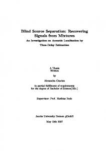
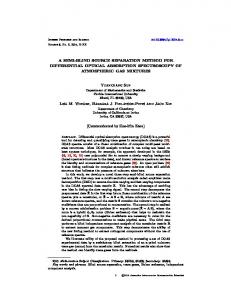
Zhirong Yang, Zhijian Yuan, and Erkki Oja Projecting high-dimensional input data into a lower-dimensional subspace is a fundamental research topic in signal processing, machine learning and pattern recognition. Nonnegative projections are desirable in many real-world applications where the original data are non-negative, consisting for example of digital images or various spectra. It was pointed out by Lee and Seung [3] that the positivity or non-negativity of a linear expansion is a very powerful constraint, that seems to lead to sparse representations for the data. Their method, non-negative matrix factorization (NMF), minimizes the difference between the data matrix X and its non-negative decomposition WH. The difference can be measured by the Frobenius matrix norm or the Kullback-Leibler divergence. Yuan and Oja [7] proposed the projective non-negative matrix factorization (PNMF) method which replaces H in NMF with WT X, thus the data matrix X is approximated as X ≈ WWT X. The nonnegative matrix W is assumed to have a much lower rank than the data matrix itself. This actually combines the objective of principal component analysis (PCA) with the non-negativity constraint. The PNMF algorithm has been applied e.g. to facial image processing, and the empirical results indicate that PNMF is able to produce more spatially localized, part-based representations of visual patterns. Recently, we have extended and completed the preliminary work with the following new contributions [5]: (1) formal convergence analysis of the original PNMF algorithms, (2) PNMF with the orthonormality constraint, (3) nonlinear extension of PNMF, (4) comparison of PNMF with two classical and two recent algorithms [6, 2] for clustering, (5) a new application of PNMF for recovering the projection matrix in a nonnegative mixture model, (6) comparison of PNMF with the approach of discretizing eigenvectors, and (7) theoretical justification of moving a term in the generic multiplicative update rule. Our in-depth analysis shows that the PNMF replacement has positive consequences in sparseness of the approximation, orthogonality of the factorizing matrix, decreased computational complexity in learning, close equivalence to clustering, generalization of the approximation to new data without heavy re-computations, and easy extension to a nonlinear kernel method with wide applications for optimization problems. Figure 3.1 demonstrates the advantage of PNMF over two other methods for the Nonnegative Kernel Principal Component Analysis problem. Furthermore, we have proposed a more general method called α-PNMF [4], using αdivergence instead of Kullback-Leibler divergence as the error measure in PNMF. We have derived the multiplicative update rules for the new learning objective. The convergence of the iterative updates is proven using the Lagrangian approach. Experiments have been conducted, in which the new algorithm outperforms α-NMF [1] for extracting sparse and localized part-based representations of facial images. Our method can also achieve better clustering results than α-NMF and ordinary PNMF for a variety of datasets. Table 3.1 shows the resulting clustering purities on six datasets.
References [1] Andrzej Cichocki, Hyekyoung Lee, Yong-Deok Kim, and Seugjin Choi. Non-negative matrix factorization with α-divergence. Pattern Recognition Letters, 29:1433–1440,
Blind and semi-blind source separation
75
(a)
(b)
0.06
0.08 POD kk−means PNMF
0.05
POD kk−means PNMF
0.07
0.06 0.04 δ value
δ value
0.05 0.03
0.04 0.03
0.02 0.02 0.01 0.01
0
iris
digit datasets
orl
0
iris
digit datasets
orl
Figure 3.1: Comparison of POD, KK-means, and PNMF with (a) linear and (b) RBF kernels for the Nonnegative Kernel Principal Component Analysis problem. Smaller δvalues are better objectives relative to the KPCA solution Table 3.1: Clustering purities using α-NMF, PNMF and α-PNMF. The best each dataset is highlighted with boldface font. α-NMF PNMF α-PNMF datasets α = 0.5 α=1 α=2 α = 0.5 α=1 Iris 0.83 0.85 0.84 0.95 0.95 0.95 Ecoli5 0.62 0.65 0.67 0.72 0.72 0.72 WDBC 0.70 0.70 0.72 0.87 0.86 0.87 Pima 0.65 0.65 0.65 0.65 0.67 0.65 AMLALL 0.95 0.92 0.92 0.95 0.97 0.95 ORL 0.47 0.47 0.47 0.75 0.76 0.75
result for
α=2 0.97 0.73 0.88 0.67 0.92 0.80
2008. [2] Inderjit Dhillon, Yuqiang Guan, and Brian Kulis. Kernel kmeans, spectral clustering and normalized cuts. In Proceedings of the tenth ACM SIGKDD international conference on Knowledge discovery and data mining, pages 551–556, Seattle, WA, USA, 2004. [3] D. D. Lee and H. S. Seung. Learning the parts of objects by non-negative matrix factorization. Nature, 401:788–791, 1999. [4] Zhirong Yang and Erkki Oja. Projective nonnegative matrix factorization with αdivergence. In Proceedings of 19th International Conference on Artificial Neural Networks (ICANN), pages 20–29, Limassol, Cyprus, 2009. Springer. [5] Zhirong Yang and Erkki Oja. Linear and nonlinear projective nonnegative matrix factorization. IEEE Transaction on Neural Networks, 2010. In press. [6] Stella X. Yu and Jianbo Shi. Multiclass spectral clustering. In Proceedings of the Ninth IEEE International Conference on Computer Vision, volume 2, pages 313–319, 2003. [7] Zhijian Yuan and Erkki Oja. Projective nonnegative matrix factorization for image compression and feature extraction. In Proc. of 14th Scandinavian Conference on Image Analysis (SCIA 2005), pages 333–342, Joensuu, Finland, June 2005.
76
3.3
Blind and semi-blind source separation
Reconstruction of historical climate data by Gaussianprocess factor analysis
Alexander Ilin and Jaakko Luttinen Studying natural variability of climate is a topic of intensive research in climatology. In our earlier research, we have extended the classical technique of rotated Principal Components, or Empirical Orthogonal Functions, by introducing the concept of “interesting structure” for massive sets of spatio-temporal climate measurements. In our case, the goal of exploratory analysis is to find signals with some specific structures of interest. They may for example manifest themselves mostly in specific variables, which exhibit prominent variability in a specific timescale etc. An example of such analysis can be extracting clear trends or quasi-oscillations from climate records. The procedure for obtaining suitable rotations of EOFs can be based on the general algorithmic structure of denoising source separation (DSS) [1]. However, understanding long-term variability of climate faces the problem of the scarcity of climate observations in the past. Thus, reconstruction of historical climate becomes an important problem. The standard methods of statistical reconstruction are ad hoc adjustments of PCA for incomplete data making such additional assumptions as temporal and spatial smoothness of the observed climate variables. These assumptions were used, for example, in [2] to reconstruct the global sea surface temperatures (SST) in the 1856–1991 period from the MOHSST5 data set (which is largely based on the measurements made from merchant ships). The method presented there uses additional information about the quality of the data and this uncertainty information is derived from the number of different sources which were used to compute each data sample. In our recent papers [3, 4], we use the Bayesian framework to perform statistical reconstructions of spatio-temporal data. In [3], we adopt the basic variational Bayesian PCA model and use additional uncertainty information to improve the reconstruction performance. In [4], we present a more advanced probabilistic model called Gaussian-process factor analysis (GPFA). The method is based on standard matrix factorization: Y = WX + noise =
D X
w:d xT d: + noise,
d=1
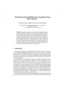
where Y is a data matrix in which each row contains measurements in one spatial location and each column corresponds to one time instance. Each xTd: is a row vector representing the time series of one of the D factors, whereas w:d is a column vector of loadings which are spatially distributed. Matrix Y may contain missing values and the samples can be unevenly distributed in space and time. We assume that both factors xd: and corresponding loadings w:d have prominent structures that we model using the tool of Gaussian processes [5]. The model is identified in the framework of variational Bayesian learning and high computational cost of GP modeling is reduced by using sparse approximations derived in the variational methodology. In the experiments reported in [4], we show that GPFA can provide better reconstructions of global SST set compared to variational Bayesian PCA. Figure 3.2 shows the spatial and temporal patterns of the four most dominant principal components found by GPFA from the MOHSST5 data set. The obtained test reconstruction errors were 0.5714 for GPFA and 0.6180 for VBPCA, which can be seen as a significant improvement.
Blind and semi-blind source separation
−0.5
0
0.5
1875
−0.5
1900
0
77
0.5
−1
1925
−0.5
0
0.5
1950
1
−0.5
0
0.5
1975
Figure 3.2: The spatial and temporal patterns of the four most dominating principal components estimated by GPFA from the MOHSST5 dataset. The solid lines and gray color in the time series show the mean and two standard deviations of the posterior distribution.
References [1] J. S¨arel¨ a and H. Valpola. Denoising source separation. Journal of Machine Learning Research, 6:233–272, 2005. [2] A. Kaplan, M. Cane, Y. Kushnir, M. Blumenthal, B. Rajagopalan. Analysis of global sea surface temperatures 1856–1991. Journal of Geophysical Research, 103:18567– 18589, 1998. [3] A. Ilin and A. Kaplan. Bayesian PCA for reconstruction of historical sea surface temperatures. In Proc. of the IEEE International Joint Conference on Neural Networks (IJCNN 2009), pp. 1322–1327, Atlanta, USA, June 2009. [4] J. Luttinen and A. Ilin. Variational Gaussian-process factor analysis for modeling spatio-temporal data. In Advances in Neural Information Processing Systems (NIPS) 22, Vancouver, Canada, Dec. 2009. [5] C. E. Rasmussen, C. K. I. Williams. Gaussian processes for machine learning. MIT Press, 2006.