Feb 8, 2001 - art of voodoo. We will examine two such .... Figure 5 shows a block diagram of the Bussgang algorithm for blind deconvolu- tion. Here:.
Blind Deconvolution and Blind Source Separation (A Summary) Shane M. Haas February 8, 2001
1
Summary
The goal of blind deconvolution and source separation is to unravel the effects of an unknown linear transformation on a unknown signal source. For blind deconvolution, the transformation is a linear finite-impulse response (FIR) filter, and for blind source separation it is a matrix of mixing coefficients. A general architecture for these blind adaptive algorithms consists of an adjustable linear transformation and a non-linear function. In this presentation, we will examine the Bussgang algorithm for blind deconvolution [2] and an informationmaximization algorithm to perform blind source separation [1].
2
Introduction Blind Deconvolution
Unknown s(n)
FIR Filter Unknown Linear Transformation
Unknown s
^ s(n)
x(n) = h n * s(n)
Matrix Multiply and Translation
Blind Adaptive Signal Processor x = Hs + h
s^
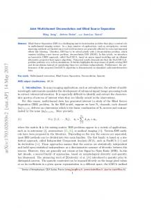
Blind Source Separation Figure 1: The blind deconvolution and blind source separation problem Figure 1 illustrates the very similar problems of blind deconvolution and blind source separation. In blind deconvolution, the goal is to recover a signal after it has passed through an FIR filter. Similarly, the goal of blind source 1
separation is to “demix” a vector of signals after they have passed through a matrix multiplication and translation operation. The problems are called “blind” because the signal processor only has access to the output of the linear transformation, and does not know the original source signal or the transformation. (InfoMax Methods) u
w
x
Adjustable Linear Transformation
Black Magic Non-Linearity
(Bussgang Methods) y
Adaptive Mechanism
Figure 2: The general architecture of a blind adaptive algorithm A general architecture for blind adaptive algorithms is shown in Figure 2. The signal passes through an adjustable linear transformation (FIR filter for blind deconvolution or matrix multiply and translation for blind source separation) and into a mysterious non-linear function. The adaptive mechanism adjusts the linear transformation in such a way as to optimize some objective function. Two pertinent questions arise: • How to choose the non-linearity? • What should the adaptive mechanism optimize? Even if we assume that the architecture shown in Figure 2 is the correct one for solving these problems, neither of these questions have definitive answers. Blind source separation and blind deconvolution are active areas of research, and many algorithms that seem to work well are ad-hoc and dabble in the subtle art of voodoo. We will examine two such algorithms in this presentation. The first method is the Bussgang algorithm for blind deconvolution [2]. It uses the celebrated Least-Mean Squares (LMS) algorithm as its adaptive mechanism and a Bayes estimator as its non-linear function. The second method, proposed by Bell and Sejnowski in [1], is sometimes called “independent component analysis.” It uses an adaptive gradient algorithm to maximize the information content of the output of a non-linear “logistic” function. It is somewhat akin to “principle component analysis” but seeks to decompose a signal into statistically independent rather than just uncorrelated components. While this algorithm can be used for both blind deconvolution and blind source separation, we will only examine its application to the blind source separation problem. 2
3
The Bussgang Algorithm for Blind Deconvolution
We will first look at the problem of blind deconvolution using the Bussgang algorithm.
3.1
The Non-Linearity: Bayes Estimator
The Bussgang algorithm for blind deconvolution uses the Bayes estimator (conditional expectation) of the source given the equalized output as its non-linear function. Let ak denote the impulse response of a filter that would ideally equalP ize the unknown FIR filter hk , i.e. k ak hn−k = δn where δn is the discrete unit impulse. We can then write the output of the adjustable FIR filter wk (n) at time n as X u(n) = wk (n)x(n − k) k
=
X k
ak x(n − k) +
X k
(wk (n) − ak ) x(n − k)
= s(n) + v(n) where s(n) is the original source signal and v(n) is the convolutional noise defined as X (wk (n) − ak )x(n − k) v(n) = k
The Bussgang algorithm uses the following approximations. Assume that v(n) is • zero-mean, • Gaussian, • white, and is • statistically independent of the source sequence s(n). This approximation is not that bad if s(n) is a sequence of independent, zeromean random variables, and the difference between the adjustable FIR filter wk (n) and the ideal equalizing filter ak is a long oscillatory sequence. If we also assume √ √that s(n) is a sequence of iid uniform random variables on the interval (− 3, 3), then the minimum mean squared error (Bayes) estimator of s(n) given u(n) is ([2], pg. 734) y(n) = E [s(n)|u(n)] =
√ √ 1 σ Z(u(n) + c0 / 3) − Z(u(n) − c0 / 3) √ √ u(n) + c0 c0 Q(u(n) − c0 / 3) − Q(u(n) + c0 / 3) 3
where σ 2 is the variance of v(n), c0 = Z(u) = Q(u) =
√
1 − σ 2 is a normalizing factor, and
u2 1 √ e− 2 2π Z ∞ z2 1 √ e− 2 dz 2π u
The reason that we assume the source is a sequence iid uniform random variables is to approximate the transmission of a real baseband M -ary pulse amplitude modulation (PAM) sequence with unit variance. To extend this result to complex baseband QAM, apply the estimator to the real and imaginary components separately ([2], pg. 741).
3.2
The Adaptive Mechanism: The LMS Algorithm
The Bussgang algorithm uses the popular LMS algorithm [2] to adjust the weights of an FIR filter. The LMS algorithm is a recursive, steepest descent approximation to the optimal Wiener filter. It tries to adjust the weights wk (n) to minimize the mean squared error between the filter output and a “desired” signal. In the Bussgang algorithm, this desired signal is the output of the Bayes estimator. w(n) k
x(n)
Adjustable FIR Filter
u(n) FIR Filter Output
LMS Algorithm
e(n) Error Signal
Σ
y(n) Desired Signal
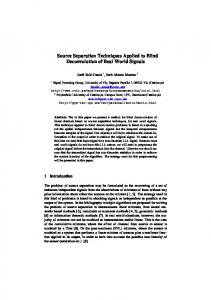
Figure 3: An adaptive filter using the LMS algorithm Figure 3 shows the structure of an adaptive filter and the LMS algorithm. The LMS algorithm adjusts the weights wk (n) to minimize the mean squared
4
error, J(n)
� � = E |e(n)|2 � � = E |y(n) − u(n)|2 � � = E |y(n) − wH (n)x(n)|2
= E[|y(n)|2 ] − wH (n)p − pH w(n) + wH (n)Rw(n)
where w(n) = (w0 (n), w1 (n), . . . , wM −1 (n))T x(n) = (x(n), x(n − 1), . . . , x(n − M + 1))T p = E[x(n)y ∗ (n)] R = E[x(n)xH (n)]
The principle of orthogonality states that the best M-tap FIR filter to minimize the mean squared error is the orthogonal projection of the desired signal onto the subspace generated by {x(n), x(n−1), . . . , x(n−M +1)}. This optimal filter w makes the error signal e(n) orthogonal to this subspace. This principle is shown graphically in Figure 4 and leads to the Wiener-Hopf condition of optimality: E[x(n)e∗ (n)] = E[x(n)(y(n) − wH x(n))∗ ] = p − Rw = 0
In other words, the optimal FIR Wiener filter, w, satisfies Rw = p This Wiener-Hopf equation can also be realized by setting the gradient of J(n), ∂J(n) = −2p + 2Rw(n) ∂w(n) equal to zero1 . Using this gradient information, we can recursively adjust the weights wk (n) to minimize J(n) in the following steepest-descent manner: ∆w
= w(n + 1) − w(n) ∂J(n) ∝ − ∂w(n) ∝ p − Rw(n)
1 We have assumed that y(n) does not depend on w; however, in the Bussgang algorithm, y(n) is the output of the Bayes estimator acting on the output of the adjustable filter. As a result, the LMS algorithm in the Bussgang algorithm is actually trying to find a minimum of a non-convex cost function that has possibly more than one minimum.
5
"Desired" Signal y(n)
Error Signal e(n)
* w0*x(n) + ... + wM-1 x(n-M+1)
Optimal Wiener Filter Projection
Subspace generated by {x(n), x(n-1), ... ,x(n-M+1)}
Figure 4: The optimal FIR filter in terms of mean squared error If we use “instantaneous” values instead of the expected values, i.e. x(n)y ∗ (n) and R ≈ x(n)xH (n), then we arrive at the LMS algorithm: ∆w
p ≈
∝ x(n)y ∗ (n) − x(n)xH (n)w(n) = x(n)(y(n) − wH (n)x(n))∗ = x(n)e∗ (n)
It can be shown ([2], pg. 317) that the LMS algorithm converges in the mean to the optimal Wiener filter if the constant of proportionality is positive and less than twice the reciprocal of the maximum eigenvalue of the covariance matrix R.
3.3
Summary of the Bussgang Algorithm
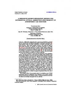
Figure 5 shows a block diagram of the Bussgang algorithm for blind deconvolution. Here: LMS Algorithm (For Complex Signals): ∆w = x(n)e∗ (n) w(n) = (w0 (n), w1 (n), . . . , wM −1 (n))T x(n) = (x(n), x(n − 1), . . . , x(n − M + 1))T e(n) = y(n) − wH (n)x(n) Bayes Estimator (Apply to Real and Imaginary Components Separately):
6
y(n) = Z(u) = Q(u) = σ2
=
c0
=
√ √ 1 σ Z(u(n) + c0 / 3) − Z(u(n) − c0 / 3) √ √ u(n) + c0 c0 Q(u(n) − c0 / 3) − Q(u(n) + c0 / 3) 1 u2 √ e− 2 2π Z ∞ z2 1 √ e− 2 dz 2π u var(v(n)) p 1 − σ2
w(n) k
x(n)
Adjustable FIR Filter
u(n)
y(n) = E[s(n)|u(n)]
y(n)
LMS Algorithm
e(n)
Σ
Figure 5: The Bussgang algorithm for blind deconvolution
4
An Information-Maximization Algorithm for Blind Source Separation
We will now examine the Bell and Sejnowski information-maximization approach to blind source separation. [1]
4.1
The Non-Linearity: The Logistic Function
As previously stated, choosing the non-linearity is somewhat of an art form. Some non-linearities work better than others on different problems. To perform blind source separation, Bell and Sejnowski use the “logistic” function yi =
1 1 + e−ui 7
where ui is the ith component of u = Wx+w, W is an adjustable N ×N matrix of demixing coefficients and w is an adjustable offset. All of these quantities are time-varying, but for notation simplicity we make this dependency implicit.
4.2
The Adaptive Mechanism: Information-Maximization
The Bell and Sejnowski algorithm adjusts the weights W and w to maximize the differential entropy of the non-linearity output. Assuming the non-linearity is an invertible function, the multivariate probability density function of its output, y, is fX (x) fY (y) = |J| where J is the Jacobian
J =
∂y1 ∂x1
···
∂y1 ∂xN
∂yN ∂x1
···
∂yn ∂xN
.. .
.. .
We can now write the differential entropy of y as h(Y)
= −E[log fY (y)] = E[log |J|] − E[log fX (x)]
The second term is a differential entropy that does not depend on the adjustable weights W and w. We will adjust the weights in a steepest ascent fashion using “instantaneous” values instead of expectations to maximize h(Y): ∆W
∝
∆w
∝
∂ log |J| ∂h(Y) ≈ ∂W ∂W ∂h(Y) ∂ log |J| ≈ ∂w ∂w
It is a rather tedious exercise in taking derivatives (see the appendix in [1] for details) but relatively straight forward to show that this adjustment rule simplifies to ∆W ∆w
4.3
∝ [WT ]−1 + (1 − 2y)xT ∝ 1 − 2y
Summary of Information-Maximization Algorithm
Figure 6 shows a block diagram of an information-maximization algorithm for blind source separation. Here: InfoMax Algorithm (For Real Signals): ∆W ∆w
∝ [WT ]−1 + (1 − 2y)xT ∝ 1 − 2y 8
Logistic Function (Apply Component-Wise): yi =
1 1 + e−ui
W,w
x
u = Wx + w
Adjustable Linear Transformation
InfoMax Adaptive Mechanism
y
y = g(u)
Figure 6: An information-maximization algorithm for blind source separation
5
Conclusions
We have examined the problems of blind deconvolution and blind source separation. For useful papers and nice demonstrations of these algorithms, see the following links: • http://www.cnl.salk.edu/˜tony/ica.html • http://sound.media.mit.edu/˜paris/ica.html • http://sweat.cs.unm.edu/˜bap/demos.html
References [1] A.J. Bell and T.J. Sejnowski. An information-maximisation approach to blind separation and blind deconvolution. Neural Computation, 7(6):1004– 1034, 1995. [2] S. Haykin. Adaptive Filter Theory. Prentice Hall, 1991.
9