Albuquerque, NM, USA. Email: {bkassiny, jayaweera, yangli}@ece.unm.edu .... to sampling, the received signal is down-converted to interme- diate frequency (IF) by ... noise process with double-sided power spectral density (PSD) of N0. 2.
IEEE ICC 2012 - Cognitive Radio and Networks Symposium
Blind Cyclostationary Feature Detection Based Spectrum Sensing for Autonomous Self-Learning Cognitive Radios Mario Bkassiny, Sudharman K. Jayaweera, Yang Li
Keith A. Avery
Dept. of Electrical and Computer Engineering University of New Mexico Albuquerque, NM, USA Email: {bkassiny, jayaweera, yangli}@ece.unm.edu
Space Vehicles Directorate Air Force Research Laboratory (AFRL) Kirtland, AFB, Albuquerque, NM, USA
Abstract—In this paper, we present an autonomous cognitive radio (CR) architecture that incorporates the main features of cognition. This model, referred to as the Radiobot, is capable of self-learning and self-reconfiguration to match its RF environment. The proposed CR architecture assumes a joint blind energy and cyclostationary detection methods to classify the communication systems in its vicinity, without any prior knowledge of the sensed signals. We derive the receiver operating characteristic (ROC) of the energy detector and show, analytically, the impact of the sliding window length on the energy detection. A learning algorithm is proposed, allowing the Radiobot to independently learn from its past experience in order to optimize its operating parameters. By applying the learning algorithm to the sensing module, we verify, through simulations, the convergence of the proposed algorithm to the optimal solution.
I. I NTRODUCTION Inspired by the concept of robots in mechanical systems, a next generation of autonomous cognitive radio (CR) architecture called the Radiobot was proposed in [1]. The notion of Radiobots goes beyond the current trend of CR which primarily aims at achieving dynamic spectrum sharing (DSS). In [1], the authors laid out a broader and more ambitious notion of autonomous radio devices that are capable of independently finding and joining/avoiding any radio network in their vicinity in order to achieve the best possible performance in any given RF environment. To achieve this, one of the most important requirements for the Radiobot is to be aware of its RF environment [1]. More particularly, the Radiobot should be able to identify/classify different activities in its vicinity by using both effective and efficient sensing, feature extraction and learning methods. For instance, by identifying the types of active communication systems and the number of users associated with each system, it makes it possible for a Radiobot to adjust its communication mode to communicate efficiently while avoiding harmful interferences, such as jammers. Moreover, by knowing the number of users in each sub-band, the Radiobot can estimate the available spectrum resources, which helps to implement efficient spectrum sensing and communication policies. Given the importance of machine learning and reconfig-
978-1-4577-2053-6/12/$31.00 ©2012 IEEE
urable hardware in the design of the Radiobots [1], we propose, in this paper, a learning algorithm that allows the Radiobot to improve its sensing techniques and adapt its design parameters based on its past experience. This allows realizing the Observe-Decide-Act-Learn (ODAL) cognition cycle of [1] and leads to the design of a real cognitive engine (CE). Different learning algorithms, such as the reinforcement learning (RL) [2], have previously been applied to CR applications to achieve autonomous cognitive behavior. The RL is an unsupervised learning algorithm that allows an agent to independently learn from past experience by trial-and-error [2]. This algorithm was applied for interference control in CR networks in [3] and for deriving distributed Medium Access Control (MAC) protocols for CR’s in [4]. The RL is suitable for Markovian environments in which it can assure certain optimal behavior [2]. In our case, however, since we do not assume any underlying Markovian framework, we propose a different unsupervised learning algorithm that allows the Radiobot to self-reconfigure its operating parameters. Our proposed algorithm is similar to that in [5] and is intended to optimize the spectrum sensing thresholds in order to achieve a desired false alarm probability. According to [5], the false alarm probability is updated during a training period in which no signals are present. In contrast, our proposed algorithm does not require a training period and can update the cyclostationary detector parameters during normal operation, whenever no signals are detected by the energy detector. Moreover, the proposed learning algorithm does not assume any prior knowledge of the observed data, and it minimizes the Kullback-Leibler distance [5] between the desired and actual performance measures. Due to the convexity of the KullbackLeibler function, the proposed algorithm is guaranteed to converge to the optimal solution, as verified in the simulations. In contrast with previously proposed MAC sensing protocols which assume prior knowledge of either the primary channels [6] or the cyclostationary properties of the sensed signals [7], our proposed Radiobot architecture assumes no such knowledge. Instead, it uses a blind joint energy and
1527
cyclostationary detection method without any prior information to identify the carrier frequencies and cyclostationarity properties of active signals. The performance of the carrier frequency detector is evaluated through its Receiver Operating Characteristic (ROC). Based on the ROC, we show analytically that the carrier frequency detection can be improved by using energy detection with a sliding window. This result was previously shown, only through simulations, in [8]. Moreover, in this paper, we develop a feature extraction algorithm that allows determining both the types and the number of users at each carrier frequency. Several signal classification and feature extraction methods have been proposed in the literature, including, for example, the model in [9] which uses support vector machines (SVM’s). In this paper, however, we employ non-parametric learning for autonomous signal identification/classification. In non-parametric approaches, models are extracted from the structures present in the data itself. Similarly to [10], we classify the extracted features based on a Chinese restaurant process (CRP). The proposed feature extraction/classification and learning are validated through simulations. The remainder of this paper is organized as follows: Section II defines the system model. Section III describes the Radiobot’s learning mechanism. We show the simulation results in Section IV and conclude the paper in Section V.
carrier frequencies and the associated cyclic frequencies that are induced by their symbol rates and coding schemes [11]. By using the discrete-frequency smoothing method described below [12], we compute an estimate of the Spectral Correlation Function (SCF) Sxα (t, f ) for a general discrete signal {x(t − M −1 kTs )}k=0 , for each sub-band. Firstly, the corresponding FFT at time t is defined as [12]:
II. S YSTEM M ODEL
The above PSD is equivalent to the sliding window energy detector that is proposed in [8]. The authors in [8] showed, through simulations, that sliding window improves the performance of energy detectors. In our paper, however, we derive in (10) of the Appendix the analytical ROC of the sliding window-based energy detector as a function of the smoothing window length L and prove that larger sliding windows lead to higher detection probability, as illustrated in Fig. 1. The active carrier frequencies in a certain sub-band are determined by setting a threshold on the above PSD. The threshold ηP SD is based on the Neyman-Pearson optimality and is derived in (9) of the Apppendix. The carrier frequencies are estimated as the midpoints of the segments formed by intersection between the PSD curve and the threshold line ηP SD . We denote by Fc the set of all detected carrier frequencies. Next, an estimate of the spectral autocoherence function magnitude [11], [12] is computed as follows:
The proposed Radiobot architecture is aimed to operate in a wideband spectrum, which is split into N sub-bands that are sensed sequentially in a round-robin style. To illustrate the same operating procedures in each and every sub-band, we consider a single sub-band and denote by N (t) the total number of signals at time t in this particular sub-band. Prior to sampling, the received signal is down-converted to intermediate frequency (IF) by using a local oscillator with frequency as fI . The corresponding h IF signal y(t) can be expressed io nP N (t) j2π (fck −fI )t [h + n(t) , y(t) = ℜ (t) ∗ x (t)] e k k k=1 where ∗ denotes the convolution, xk (t) denotes the baseband signal of user k using carrier frequency fck , and hk (t) denotes the baseband equivalent channel impulse response of the channel between the user k and the Radiobot. The receiver noise is denoted by n(t), which is assumed to be a white noise process with double-sided power spectral density (PSD) of N20 . The average noise power at the output of the sweeping IF filter will thus be Pn = N20 B , where B is the IF filter bandwidth. The resulting signal-to-noise ratio (SNR) at the output of the IF filter is SN R = PPns , where Ps is the received T signal power. We denote by y = [y(1), · · · , y(M )] an M length vector of the sampled discrete-time IF signal, such that y(k) = y(kTs ), for k ∈ {1, · · · , M }, where Ts is the sampling period. A. Identification of RF Activities We apply a cyclostationarity-based signal detection to the sensed vector y in order to identify the RF activity in the sub-band of interest. We identify the active signals by their
˜ f) = X(t,
M −1 X
a(t − kTs )x(t − kTs )e−j2πf (t−kTs ) ,
(1)
k=0
where a(t) is a triangular data tapering window. The FFT ˜ f ) is defined over the set of frequencies {− fs , − fs + X(t, 2 2 Fs , · · · , f2s − Fs , f2s }, where fs = T1s and Fs = M1Ts is the frequency increment. An approximation to the SCF is [12]: 1 S˜xα (t, f ) = LT
(L−1)/2
X
ν=−(L−1)/2
˜ f + α +νFs )X ˜ ∗ (t, f − α +νFs ), X(t, 2 2
where T = M Ts is the time length of the data segment, α is the cyclic frequency and L (an odd number) is the spectral smoothing window length. By setting α = 0, we may obtain an −1 estimation of the PSD of the discrete signal {x(t−kTs )}M k=0 : 1 S˜x0 (t, f ) = LT
˜xα (t, f )| = q |C
(L−1)/2
X
ν=−(L−1)/2
¯2 ¯ ¯ ¯˜ ¯X(t, f + νFs )¯ .
|S˜xα (t, f )|
(2)
.
(3)
S˜x0 (t, f + α/2)S˜x0 (t, f − α/2)
We denote the cyclic sub-domain profile of carrier frequency fc ∈ Fc as I˜x (t, α, fc ) = maxf ∈[fc −∆fL ,fc +∆fU ] |C˜xα (t, f )|, where fc − ∆fL and fc + ∆fU are the lower, and upper limit of the considered frequency range for carrier frequency fc , respectively. In [11], it is shown that digital signals exhibit cyclostationarity at multiples of their symbol rates. Moreover, the digital signals may exhibit other periodicities as well: For example, due to coding. We denote the RF signature of the signal centered at fc as RF(fc ) = {α 6= 0 : IE I˜x (t, α, fc ) ≥ ζ},
1528
where IE denotes the indicator function of event E = {I˜x (t, α, fc ) is a local maximum}, and ζ ∈ (0, 1). It is hard to derive, analytically, an optimal choice for the parameter ζ due to the complexity of the cyclic sub-profile function and the environment randomness. However, as we show in Section III, we apply a learning algorithm to optimize the value of ζ for any unknown environment. B. Feature Extraction Method We define a feature extraction method that helps to estimate the number of distinct signals at each carrier frequency. This method estimates the number of periodic-peaks sequences in each cyclic sub-profile that is centered at carrier frequency fc . According to the periodicity properties of the cyclic subprofiles, if a signal exhibits a cyclic component at a certain cyclic frequency α, then it also exhibits cyclic components at integer multiples of α. Thus, each periodic-peaks sequence corresponds to at least one communication signal type. By detecting the number of periodic-peaks sequences in a certain cyclic sub-profile, we may determine the minimum number of distinct communication signals that are transmitted simultaneously at each carrier frequency1 . Each of those detected signal is represented by its carrier frequency fc and its fundamental cyclic frequency component α, thus defining a 2-D feature space for identifying the minimum number of users at each carrier frequency2 . The detected features will be classified in a 2-D feature space based on the CRP, similar to [10]. III. S ELF -R ECONFIGURATION OF THE S PECTRUM S ENSING M ODULE The performance of the Radiobot is related to the quality and accuracy of the sensing observations. It is required to optimize the sensing module so that it best estimates the RF activity in the surrounding environment. Several parameters may need to be optimized during the sensing process, such as the sensing duration, detector thresholds, spectrum sensing policies, etc. based on the particular RF environment it encounters at a given time. Due to its learning and reasoning abilities, the Radiobot can dynamically adapts these parameters based on its past experience. To be specific, assume that the Radiobot needs to optimize its cyclic sub-profile threshold ζ such that it achieves a certain false alarm probability. It is very hard to obtain analytical solutions to this problem due to the complexity of the cyclic profile equation and to the uncertainty in the surrounding environment. A possible solution is to learn the optimal threshold value iteratively based on the sensing observations, as in [5]. An online learning algorithm was proposed in [5] to adapt the threshold value of Neyman-Pearson test when the probability distribution of the detected signals is unknown. The threshold is thus dynamically updated to achieve a desired 1 Including
primary users, interferers and cognitive secondary users. 2 The feature space can be extended to higher dimensions to account for other signal features, such as the direction of arrival. This allows to discriminate between simultaneous transmissions having the same carrier frequency, symbol rate and coding rate.
false alarm probability. The learning process is conducted during a training period in which the observed data are drawn from a null hypothesis. In our case, however, we do not assume a training period and we propose a learning algorithm that updates the cyclic sub-profile threshold ζ during the normal operation time itself to achieve a desired false alarm probability φ. By the help of the energy detection, the learning algorithm identifies the absence of transmitted signals to perform the learning process. The objective of the learning algorithm is to minimize the Kullback-Leibler distance K(P ||Q) between two probability distributions P and Q, similar to [5], where: X P (i) K(P ||Q) = . P (i) log Q(i) i We denote by P and Q the desired and actual probability distributions of the cyclostationary detector output, conditioned on the absence of transmitted signals. These probability distributions correspond to Bernoulli random variables, representing whether a signal is (1) or is not (0) detected. By defining φ and Pf (ζ) as the desired and actual false alarm probabilities (for a given threshold ζ), respectively, the Kullback-Leibler distance can then be expressed as: K(P ||Q) = K(φ, Pf (ζ)) = φ log
1−φ φ +(1−φ) log . Pf (ζ) 1 − Pf (ζ)
The Kullback-Leibler distance K(φ, Pf (ζ)) is a nonnegative quantity representing the difference between φ and Pf (ζ), with K(φ, Pf (ζ)) = 0 if and only if φ = Pf (ζ). Due to its convexity in Pf (ζ), the Kullback-Leibler distance guarantees a global minimum and makes a perfect candidate for convex optimization problems. Moreover, it was shown in [5] that K(φ, Pf (ζ)) is convex in ζ if and only if Pf (ζ) is monotonous, which is satisfied in our case. However, since the analytical expression of Pf (ζ) is unknown, it can be estimated as the ratio of sample points that exceed the threshold ζ in the cyclic profile I(α), when there is no transmitted signals. As noted in [5], to achieve accurate estimate for Pf (ζ), the recursive adaptation in ζ should not be too frequent. This Algorithm 1 Learning algorithm to control the cyclic subprofile threshold ζ Initialize: counter = 1. while No signal is detected by the energy detector do Update the false alarm probability Pf (ζ) and counter = counter + 1. if counter = Nc then Update ζ such that: ζ ← ζ + ψ (Pf (ζ) − φ). Reset counter = 1. end if end while
is taken into account in the proposed learning algorithm (Algorithm 1), in which the threshold ζ is updated after each Nc > 1 updates of the false alarm probability Pf (ζ). The value of Nc is selected such that it achieves convergence of the estimated false alarm probability Pf (ζ).
1529
Receiver Operating Charcteristic (ROC) for carrier frequency detection with SNR= 0 dB
14
1 0.9
12 Cyclic Frequency (α1) in MHz
0.8
Detection Probability P
D
0.7 0.6 0.5 0.4 0.3
Sliding Window Energy Detection: L= 11 (Analytical) Sliding Window Energy Detection: L= 11 (Simulation) Sliding Window Energy Detection: L= 3 (Analytical) Sliding Window Energy Detection: L= 3 (Simulation) Conventional Energy Detection: L= 1 (Analytical) Conventional Energy Detection: L= 1 (Simulation)
0.2 0.1 0 0
0.1
0.2
0.3
0.4 0.5 0.6 False Alarm Probability (α)
0.7
0.8
0.9
10
8
6
4
2
0 76
1
Fig. 1. The impact of the sliding window length L on the ROC of the carrier frequency detector.
78
80 82 84 Carrier Frequency (fc) in MHz
86
88
Fig. 2. Detection and CRP-based classification of simultaneous system transmissions at a single carrier frequency. Learning curves of the cyclic sub−profile threshold ζ and the false alarm probability P with ψ= 0.2 f
1
The update rule in Algorithm 1 minimizes the KullbackLeibler function since it follows a gradient descent direction that reduces the difference |Pf (ζ) − φ| at a learning rate of ψ > 0. Moreover, due to the convexity of the Kullback-Leibler function, this algorithm is guaranteed to converge to a unique optimal threshold value.
0.9 0.8 0.7 0.6 0.5 0.4
IV. S IMULATION R ESULTS
ζ: φ= 0.01 ζ: φ= 0.1 P : φ= 0.1
0.3
First, we show, in Fig. 1, the performance comparison between the sliding window-based (L > 1) and conventional (L = 1) energy detections. The ROC’s of Fig. 1 show that higher detection probabilities can be achieved for larger sliding window length L. Next, in order to verify the proposed signal classification and learning techniques, first, we assume two arbitrary users that are operating in the sensed sub-band of interest. These users are assumed to transmit simultaneously at a WiFi channel centered at f1 = 2.437GHz. Their transmit signals are sensed and downconverted to an intermediate frequency (IF) by using a local oscillator of 2.35GHz (chosen such that the IF signal can be sampled using a realistic ADC). We assume that the first user uses a symbol rate of 14Mbauds and the second system uses 12Mbauds with a coding rate of 1/2. In each sensing period of 12µs, the feature points (fc , α) are detected and classified into clusters based on the CRP [10]. Figure 2 shows the clusters after 20 sensing periods. We notice two major clusters (in bold circles) which occur with a probability higher than 0.1. These clusters are distributed around fc = 87MHz, representing the carrier frequency after IF conversion. The cluster with α = 6MHz corresponds to the signal of 12Mbauds with a coding rate of 1/2, and the other cluster at α = 14MHz corresponds to the uncoded signal of 14Mbauds. Next, we verify, in Fig. 3, the convergence of the learning algorithm proposed in Section III. We let φ to be the desired false alarm probability of the cyclostationary detection and let ζ be the control threshold. Starting from ζ = 0, Algorithm 1 converges to constant threshold at which the actual false alarm probability Pf (ζ) converges to φ. The learning rate is set to ψ = 0.2 and the threshold ζ is updated after each Nc = 20 updates of the false alarm probability Pf (ζ).
f
0.2
Pf: φ= 0.01
0.1 0
2
4
6
8
10 12 Iteration Number
14
16
18
20
Fig. 3. Learning curves of the cyclic sub-profile threshold ζ and the false alarm probability Pf with a learning rate ψ = 0.2 and a desired false alarm probability φ.
This result shows that the proposed learning algorithm can accurately reconfigure the Radiobot’s parameters and helps achieving the desired performance levels. V. C ONCLUSION In this paper, we have proposed an autonomous sensing architecture for a futuristic autonomous CR, referred to as the Radiobot [1]. The proposed system applies a blind cyclostationary detection method to identify/classify the active users in the RF environment. An ROC was derived showing that energy detection can be improved by using sliding window averaging techniques. We developed an unsupervised learning mechanism that allows the Radiobot to learn from its past experience and to self-reconfigure its sensing parameters. We showed, through simulations, that the proposed learning algorithm optimizes the Radiobot’s parameters in order to achieve a desired objective. ACKNOWLEDGMENT This research was supported in part by the National Science foundation (NSF) under the grant CCF-0830545 and the Space Vehicles Directorate of the Air Force Research Laboratory (AFRL), Kirtland AFB, Albuquerque, NM.
1530
determine the distribution of T (n) under the two hypotheses:
R EFERENCES [1] S. K. Jayaweera and C. G. Christodoulou, “Radiobots: Architecture, algorithms and realtime reconfigurable antenna designs for autonomous, self-learning future cognitive radios,” University of New Mexico, Technical Report EECE-TR-11-0001, Mar. 2011. [Online]. Available: http://repository.unm.edu/handle/1928/12306 [2] R. S. Sutton and A. G. Barto, Reinforcement Learning: An Introduction. Cambridge, MA: MIT Press, 1998. [3] A. Galindo-Serrano and L. Giupponi, “Distributed Q-Learning for aggregated interference control in cognitive radio networks,” IEEE Transactions on Vehicular Technology, vol. 59, no. 4, pp. 1823 –1834, May 2010. [4] M. Bkassiny, S. K. Jayaweera, and K. A. Avery, “Distributed reinforcement learning based mac protocols for autonomous cognitive secondary users,” in 20th Annual Wireless and Optical Communications Conference (WOCC ’11), Newark, NJ, Apr. 2011, pp. 1 –6. [5] D. Pados, P. Papantoni-Kazakos, D. Kazakos, and A. Koyiantis, “Online threshold learning for neyman-pearson distributed detection,” IEEE Transactions on Systems, Man and Cybernetics, vol. 24, no. 10, pp. 1519 –1531, Oct. 1994. [6] J. Unnikrishnan and V. Veeravalli, “Algorithms for dynamic spectrum access with learning for cognitive radio,” IEEE Transactions on Signal Processing, vol. 58, no. 2, pp. 750–760, Feb. 2010. [7] J. Lunden, V. Koivunen, A. Huttunen, and H. Poor, “Collaborative cyclostationary spectrum sensing for cognitive radio systems,” IEEE Transactions on Signal Processing, vol. 57, no. 11, pp. 4182 –4195, Nov. 2009. [8] Y. M. Kim, G. Zheng, S. H. Sohn, and J. M. Kim, “An alternative energy detection using sliding window for cognitive radio system,” in 10th International Conference on Advanced Communication Technology (ICACT ’08), vol. 1, Gangwon-Do, South Korea, Feb. 2008, pp. 481 – 485. [9] M. Ramon, T. Atwood, S. Barbin, and C. Christodoulou, “Signal classification with an SVM-FFT approach for feature extraction in cognitive radio,” in SBMO/IEEE MTT-S International Microwave and Optoelectronics Conference (IMOC ’09), Belem, Brazil, Nov. 2009, pp. 286 –289. [10] N. Shetty, S. Pollin, and P. Pawelczak, “Identifying spectrum usage by unknown systems using experiments in machine learning,” in IEEE Wireless Communications and Networking Conference (WCNC ’09), Budapest, Hungary, Apr. 2009, pp. 1 –6. [11] W. Gardner, W. Brown, and C.-K. Chen, “Spectral correlation of modulated signals: Part ii–digital modulation,” IEEE Transactions on Communications, vol. 35, no. 6, pp. 595 – 601, June 1987. [12] W. Gardner, “Measurement of spectral correlation,” IEEE Transactions on Acoustics, Speech and Signal Processing, vol. 34, no. 5, pp. 1111 – 1123, Oct. 1986. [13] H. V. Poor, An Introduction to Signal Detection and Estimation, 2nd ed. New York: Springer, 1998, ch. 3, pp. 72–76. [14] F. Millioz and N. Martin, “Estimation of a white gaussian noise in the short time fourier transform based on the spectral kurtosis of the minimal statistics: Application to underwater noise,” in IEEE International Conference on Acoustics Speech and Signal Processing (ICASSP ’10), Dallas, TX, Mar. 2010, pp. 5638 –5641.
A PPENDIX D ERIVATION OF THE T HRESHOLD AND THE ROC FOR C ARRIER F REQUENCY D ETECTION −1 Consider a sampled data sequence {x(k)}M k=0 , with Ts as M −1 the sampling period. We denote by {X(n)}n=0 its discrete Fourier transform (DFT) obtained by FFT:
X(n) =
M −1 X
H0 : x(k) H1 : x(k)
x(k)e
, for n = 0, · · · , M − 1.
(4)
k=0
The average power in a spectral window of odd length L, centered at n, can be approximated by T (n) = P(L−1)/2 2 l=−(L−1)/2 |X(n+l)| . In order to derive the receiver operating characteristic (ROC) of the Neyman-Pearson detector, we
(5) (6)
M −1 where {w(k)}k=0 are modeled as i.i.d. Gaussian random M −1 variables, s.t. w(k) ∼ N(0, Pn ). The signal {s(k)}k=0 in (6) can be modeled as i.i.d. Gaussian random variables, s.t. s(k) ∼ N(0, Ps ). This is a reasonable assumption for signals that are perturbed by propagation through turbulent media and multipath fading [13]. It is well-known that the energy detector is the optimal detector for unknown (random) signals. Let x = [x(0), · · · , x(M − 1)]T , X = [X(0), · · · , X(M − 1)]T , XR = [ℜ{X(0)}, · · · , ℜ{X(M − 1)}]T and XI = [ℑ{X(0)}, · · · , ℑ{X(M −1)}]T , , where ℜ{} and ℑ{} denote the real and imaginary parts, respectively. The DFT in (4) can be expressed as:
XC ,
·
XR XI
¸
= Ax ,
(7)
where A is a 2M -by-M matrix of DFT coefficients. Since −1 {x(k)}M k=0 are zero-mean i.i.d. Gaussian random variables, C then X is a jointly Gaussian vector. It can be shown ¡ C ¢Trandom M Pn C } = 2 IM (where IM is an that, under H0 , E{X X ¡ ¢T M -by-M identity matrix) and under H1 E{XC XC } = M (Ps +Pn ) IM . Therefore, elements of XC are uncorrelated. 2 Since XC is jointly Gaussian with uncorrelated elements, the elements of XC are then independent. Also, since all the elements have the same variance under the same hypothesis, elements of XC are assumed to be i.i.d. zero-mean Gaussian random variables with variance M2Pn under H0 , and M (Pn +Ps ) under H1 . 2 Under the above assumptions, T ′ (n) = M2Pn T (n) is a sufficient statistic for the hypothesis testing and follows a χ22L distribution. The threshold η for carrier frequency detection is defined s.t. Pr{T ′ (n) > η|H0 } ≤ αF , where αF is the acceptable false alarm probability. Note that the noise power Pn can be estimated, for example, by using the method proposed in [14]. The Neyman-Pearson decision rule δ for carrier frequency detection is then defined as: ½ 0 if T ′ (n) < η ′ , (8) δ (T (n)) = 1 otherwise where η = 2γ −1 (L; (1 − αF ) Γ(L)), γ −1 is the Rinverse lower x incomplete gamma function (where γ(k; x) = 0 tk−1 e−t dt and inverse is w.r.t. the second argument) and Γ(k) = R ∞ the k−1 −t t e dt is the gamma function. By applying this to the 0 PSD in (2), the threshold is given by: ηP SD =
k −j2πn M
= w(k), = s(k) + w(k),
γ −1 (L; (1 − αF ) Γ(L)) Pn ηPn = . 2Ts L Ts L
(9)
The resulting detection probability of this detector can be expressed as: PD = Pr{T ′ (n) > η|H 1 } = 1 −
³ γ L;
η 2(1+SN R)
Γ(L)
´
,
(10)
which represents the ROC of the carrier frequency detector.
1531