Blind Deconvolution of Images using Optimal Sparse Representations

SUBMITTED FOR REVIEW TO IEEE TRANSACTIONS ON IMAGE PROCESSING

1

Blind Deconvolution of Images using Optimal Sparse Representations Michael M. Bronstein*, Student Member, IEEE, Alexander M. Bronstein, Student Member, IEEE, Michael Zibulevsky, Member, IEEE, and Yehoshua Y. Zeevi

Abstract— The relative Newton algorithm, previously proposed for quasi maximum likelihood blind source separation and blind deconvolution of one-dimensional signals is generalized for blind deconvolution of images. Smooth approximation of the absolute value is used in modelling the log probability density function, which is suitable for sparse sources. In addition, we propose a method of sparsification, which allows blind deconvolution of sources with arbitrary distribution, and show how to find optimal sparsifying transformations by training. Index Terms— blind deconvolution, quasi maximum likelihood, sparse representations, relative Newton optimization.

I. I NTRODUCTION

T

WO-dimensional blind deconvolution (BD) is a special case of a more general problem of image restoration. The goal of BD is to reconstruct the original scene from an observation degraded by the action of a linear shift invariant (LSI) system, when no or very little a priori information about the scene and the degradation process is available, hence the term ”blind”. BD is critical in many fields, including astronomy [1], [2], remote sensing [3], biological and medical imaging [4], [5] and microscopy [6], [7]. Typically, the image is degraded by imperfections of an optical system, and can be presented in terms of convolution of the source image with some blurring kernel or point spread function (PSF); in such applications, the term deblurring is synonymous to deconvolution. A. Problem formulation In the general setup of 2D BD, the observed sensor image X is created from the source image S passing through a convolutive system defined by its impulse response W , X Xmn = Wkl Sm−k,n−l + Umn , k,l

and is possibly contaminated by additive sensor noise U . We assume that the action of W is invertible, at least approximately. The aim of BD is to find such deconvolution Manuscript received October 10, 2003. This research has been supported by the HASSIP Research Network Program HPRN-CT-2002-00285, sponsored by the European Commission. Asterisk indicates corresponding author. M. M. Bronstein is with the Department of Computer Science, Technion – Israel Institute of Technology, Haifa 32000, Israel. A. M. Bronstein, M. Zibulevsky and Y. Y. Zeevi are with the Department of Electrical Engineering, Technion – Israel Institute of Technology, Haifa 32000, Israel (e-mail: [email protected]; [email protected]; [email protected]; [email protected]).

(restoration) kernel H that produces an estimate S˜ of S up to integer shift and scaling factor c: X S˜mn = Hkl Xm−k,n−l ≈ c · Sm−∆M ,n−∆N , k,l

or equivalently, the global system response should be Gmn

= (W ∗ H)mn ≈ c · δm−∆M ,n−∆N ,

where δij denotes the Kr¨onecker delta (discrete impulse signal). B. Previous work Various BD methods have been previously proposed. We will only briefly outline the basic approaches (for a comprehensive comparison see e.g. [8]). Most of the BD approaches can be divided into parametric and non-parametric. In applications where the form of the PSF can be assumed in advance (e.g. motion blur or defocus), it is possible to use a parametric model of the PSF and instead of finding the PSF itself, one can try to estimate the parameters of its model. In real applications it is often difficult to derive a good model for the PSF; the advantages are, obviously, in having a smaller number of variables. BD approaches can be divided into those that estimate the blurring kernel, those estimating the source image and the blurring kernel simulataneously, and those estimating the restoration kernel. The first class includes the so-called a priory blur identification methods, which first estimate the blurring kernel and then employ a non-blind deconvolution algorithm to find the source estimate [9]–[11]. The second class includes methods based on statistical or deterministic priors of the source image, the blurring kernel and the noise [12], [13]. Estimation of the source image is performed by maximizing some optimality criterion, which includes these priors. Since the variables in this problem are both the source image and the blurring kernel, the computational complexity is a major problem. The third class of methods usually employs maximum likelihood (ML) estimators of the restoration kernel; such estimators can incorporate priors on the image and the kernel. Since there is no need to estimate the source image, these approaches demand the solution of more modest optimization problems and, consequently, are much more efficient. However, the exact source distribution, required for the ML approach, is often unknown. A possible remedy is to use an approximate probability density function; such a modified ML approach is usually

SUBMITTED FOR REVIEW TO IEEE TRANSACTIONS ON IMAGE PROCESSING

2

referred to as quasi ML (QML). Such estimation techniques were successfully used in blind source separation (BSS) [14]– [16]. The relative Newton quasi ML framework for BD of 1D signals was introduced in [17]. Here, we extend it to the 2D case. In addition, we present a novel approach of using optimal sparse representation, which can be used for BD of source images with arbitrary distributions.

where λ is a positive smoothing parameter [15]; ϕλ (t) → |t| as λ → 0+ . For convenience, we henceforth omit λ from our notation whenever possible, and refer to ϕλ (·) without using the subscript. Yet another important advantage of working with superGaussian sources is the fact that the asymptotic restoration error variance is significantly smaller compared to sub-Gaussian sources, i.e., deconvolution is more accurate. This issue is addressed in [18].

II. Q UASI ML BLIND DECONVOLUTION The convolution operation H ∗ X can be thought of as application of an infinite Toeplitz block-Toeplitz operator H, defined by the impulse response Hmn . Denoting the source estimate by Y = H ∗ X and assuming that S is i.i.d., the following minus-log likelihood function of the observed signal X, given the restoration kernel H is obtained in the case of zero noise [18]: L(H; X) = Z Z ¯ ¯ X MX NX π π ¯ˆ ¯ − ϕ(Ymn ), (1) log H(ξ, η) dξdη + ¯ ¯ 4π 2 −π −π m,n where MX NX is the observation sample size, ϕ(·) = − log pS (·), and pS (·) stands for the source probability density function (PDF). X ˆ η) = H(ξ, Hmn e−i(mξ+nη) m,n

denotes the Fourier transform of Hmn . We will henceforth assume that Hmn has finite impulse response (FIR), supported on [−M, ..., M ] × [−N, ..., N ]. We will use KM = 2M + 1 and KN = 2N + 1 to denote the dimensions of the restoration kernel.

B. Approximation of the log-likelihood function using FFT In practice, the first term of L(H; X), containing the integral, is difficult to evaluate. It can, however, be approximated with any desired accuracy by [17] Z π Z π ¯ ¯ 1 ¯ˆ ¯ log ¯H(ξ, η)¯ dξdη ≈ 2 4π −π −π MF X NF ¯ ¯ X 1 ¯ˆ ¯ log ¯H kl ¯ , MF NF k=0 l=0

where

µ ˆ kl H

=

ˆ FMF ,NF {Hmn }kl = H

f1

distributions lead to non-convex prior term in the minus log-likelihood function. 2 Super-Gaussian sources are defined as signals possessing positive kurtosis excess IEx4 /IE2 x2 − 3. Sub-Gaussian sources have negative kurtosis excess.

(3)

=

MF X NF X

¯ ¯ ¯ ˆ ¯2 log ¯H kl ¯

(4)

k=0 l=0

=

X

ϕ(Ymn ),

(5)

m,n

A. The choice of ϕ(·)

1 Non-log-concave

¶

are the 2D DFT coefficients of Hmn , zero-padded to the support MF × NF . F denotes the 2D FFT operator. The approximation error vanishes as MF , NF grow to infinity. Choosing MF and NF as integer powers of 2, allows to use 2D FFT. For convenience, we denote

f2 Natural images encountered in most applications are usually characterized by non-log-concave, multi-modal distributions, which are difficult to model and are not well-suited for optimization1 . However, consistent estimator of S can be obtained by minimizing L(H; X) even when ϕ(·) is not exactly equal to − log pS (·). Such quasi ML estimation has been shown to be practical in instantaneous BSS [14], [16], [19] and BD of 1D signals [17], [20]. For example, when the source is superGaussian2 (e.g. it is sparse or sparsely representable), a smooth approximation of the absolute value function is a good choice for ϕ(·) [17], [19], [21]. Although natural images are usually far from being sparse, they can be sparsely represented by a proper transformation [16], [22]. (In Section IV, we will show how to transform general classes of natural images into sparse ones.) We therefore focus our attention on modelling super-Gaussian distributions using a family of convex smooth functions ¶ µ |t| , (2) ϕλ (t) = |t| − λ log 1 + λ

2πk 2πl , MF NF

and define the approximate normalized minus-log likelihood function as 1 1 f1 (H) + f2 (Y ). (6) L(H; X) = − 2MF NF MX NX C. Gradient and Hessian of L(H; X) Optimization algorithms discussed in Section III-C require the knowledge of the gradient and the Hessian of L(H; X). Since the optimization variable H is a KM × KN matrix, the gradient ∇L is also a KM × KN matrix, whereas the Hessian ∇2 L is a KM × KN × KM × KN fourth-order tensor. For convenience, we parse the variables column-wise into a KM KN × 1 vector £ ¤T H−M,−N , ..., HM,−N , ..., HM,N , vec(H) = and define the gradient and the Hessian of L(H; X) as a KM KN × 1 vector and a KM KN × KM KN matrix, respectively. The gradient of f1 is given by ∇f1

= vec (Q0kl + Q0∗ kl ) ,

and the i-th row of the Hessian of f1 is ¡ 2 ¢ ¡ ¢ ∇ f1 i = vec Q00k+k0 ,l+l0 + Q00∗ k+k0 ,l+l0 ,

(7)

SUBMITTED FOR REVIEW TO IEEE TRANSACTIONS ON IMAGE PROCESSING

where Q0kl Q00k+k0 ,l+l0

n o −1 ˆ mn = FMF ,NF H kl n o −2 ˆ = −FMF ,NF Hmn

k+k0 ,l+l0

,

i−1 and k 0 = (i − 1) mod KM − M and l0 = b K c − N . The M gradient and the i-th row of the Hessian of f2 are given by

∇f2 ¡ 2 ¢ ∇ f2 i

=

vec ((Φ0 ∗ J X)kl ) ,

= vec

³³ 0 0 ´ ´ Ak l ∗ J X ,

(8)

kl

0 0

respectively, where Φ0mn = ϕ0 (Ymn ), Akmnl = 00 ϕ (Ymn ) · Xm−k0 ,n−l0 , (J X)mn = XMX −m,NX −n , i−1 k 0 = (i − 1) mod KM − M , and l0 = b K c − N. M (For derivation see [18].) Computational complexity of the target function L and its gradient is O(MF NF log2 MF NF + MX NX log2 MX NX ); whereas evaluation of the Hessian requires O(MF NF log2 MF NF + M N MX NX log2 MX NX ) operations.

3

on G(k−1) = W ∗ H (k−1) . This property follows in a straightforward manner from the definition of the relative optimization algorithm. Equivariance implies that for any invertible kernel ˜ A, the estimator H(X) of the restoration kernel H given the observation X, obtained by minimization of the target function L(H; X) obeys [18] ˜ H(A ∗ X)

˜ = A−1 ∗ H(X),

i.e., the parameters to be estimated (in our case, coefficients Hmn of the restoration kernel) form a group. This is indeed the case for invertible kernels with the convolution operation. It must be noted, however, that when the restoration filter support is limited by cropping, equivariance holds only approximately.

B. Newton method Newton method is often used for unconstrained optimization, since it provides a very fast (quadratic) rate of convergence. In this approach, the direction d at each iteration is given by solution of the linear system [23] ∇2 L · d = −∇L.

III. R ELATIVE N EWTON ALGORITHM A fast relative optimization algorithm for BSS, based on the Newton method, was introduced in [15] as a modification of the approach presented in [14]. This method was extended in [17] to BD of time series. Here, we extend these results to BD of images. A. Relative optimization algorithm The main idea of relative optimization is to iteratively produce source estimate and use it as the current observation. This yields the following algorithm: Relative optimization algorithm 1) Start with H (0) , and with X (0) = X. 2) For k = 1, 2, ..., until convergence 3) Compute current source estimate: X (k) = H (k−1) ∗ X. (k) 4) Starting with Vmn = δmn , compute coefficients of the restoration kernel, which sufficiently decrease L(H = V (k) ; X (k) ). 5) H (k) = V (k) ∗ H (k−1) . 6) End For This method allows to construct large restoration kernels of the form H

= H (0) ∗ H (1) ∗ ... ∗ H (K−1)

(9)

using a set of low-order factors (K denotes the number of relative optimization iterations). The algorithm assumes infinite memory and produces a restoration kernel of order growing at each iteration. In real applications it might be necessary to limit the support of the restoration kernel. This can be done by cropping the kernel obtained in Step 5. Another remarkable property of the relative optimization algorithm is its equivariance: the relative optimization algorithm is equivariant, i.e. its step at iteration k depends only

(10)

Since the objective function is non-convex, in order to guarantee descent direction, positive definiteness of the Hessian is forced by using modified Cholessky factorization [23]. Having the direction d, the new iterate h(k+1) is given by h(k+1)

=

h(k) + α(k) d,

where α(k) is the step size determined, e.g., by backtracking line search restricted to the subspace where the inverse of the restoration kernel is stable, i.e. log | det H| > −∞ [18]. Newton method is used in Step 4 of the relative optimization algorithm [15], [17]; such an optimization algorithm will be referred to as the relative Newton method. Apart from gradient and Hessian evaluation, required at each relative Newton 3 3 2 2 iteration, additional O( 16 KM KN + KM KN ) operations are required for solution of the Newton system (10) using modified Cholessky factorization [23].

C. Fast relative Newton step Practical use of the relative Newton step is limited to cases of small M, N, MX , NX , due to the complexity of Hessian construction and solution of the Newton system. This complexity can be significantly reduced if special Hessian structure at the minimum is exploited. ˆ ≡ 1, from where Substituting Hmn = δmn to (7) yields H ¯ ¯ ∂ 2 f1 ¯ = ∂Hkl ∂Hk0 l0 ¯Hmn =δmn n o n o −2 −2 ˆ mn ˆ mn −F H − F∗ H 0 0 k+k0 ,l+l0

=

k+k ,l+l

−2MF NF δk+k0 ,l+l0 .

It can be easily seen that ∇2 f1 is a constant anti-diagonal matrix with −2MF NF on the secondary diagonal. Therefore, f1 contributes a unit anti-diagonal to ∇2 L.

SUBMITTED FOR REVIEW TO IEEE TRANSACTIONS ON IMAGE PROCESSING

4

1

1

1

4

4

4

7

7

7

For Hmn = δmn and X = c · S, one obtains Y = c · S. Substituting to (8) yields ∂ 2 f2 = ∂Hkl ∂Hk0 l0 X c2 · ϕ00 (c · Smn ) Sm−k,n−l Sm−k0 ,n−l0 . m,n

1

4

7

(a)

For sufficiently large MX , NX , ∂ 2 f2 ≈ ∂Hkl ∂Hk0 l0 c2 MX NX · IE {ϕ00 (c · Smn ) Sm−k,n−l Sm−k0 ,n−l0 } .

1

4

7

(b)

1

4

7

(c)

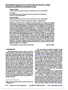
Fig. 1. Hessian structure for Hmn = δmm with M = N = 1 (3 × 3 kernel): (a) diagonal-anti-diagonal form for γσ 02 ≈ 10; (b) anti-diagonal form for γσ 02 ≈ 10−6 ; (c) diagonal form for γσ 02 ≈ 106 . White stands for near-zero elements of the matrix.

Without loss of generality, let us assume that Smn is zeromean. Since S is i.i.d., ∂ 2 f2 ≈ ∂Hkl ∂Hk0 l0   αc2 γσ 02 MX NX ·  0

: k = k 0 = l = l0 = 0 : k = k 0 6= 0, l = l0 6= 0 : otherwise,

where α = c2 · IEϕ00 (c · S)S 2 , γ = IEϕ00 (c · S), σ 2 = IES 2 , and σ 0 = cσ. We conclude that ∇2 L(H = δmn ; c · X) has an approximate diagonal-anti-diagonal form. When γσ 02 À 1, ∇2 L(H = δmn ; c · X) is approximately diagonal. When γσ 02 ¿ 1, ∇2 L(H = δmn ; c · X) has an approximate anti-diagonal form. Hessian structure is visualized in Figure 1 for different ranges of γσ 02 . When γ 2 σ 04 < 1, the Hessian at the solution point is not positive-definite, which means that the QML estimator is asymptotically unstable. This issue is addressed in depth in [18]. Using the diagonal approximation, which is valid for γσ 02 À 1, the Newton system (10) can be solved as a set of KM KN independent linear equations dk

=

−

(∇L)k , (∇2 L)kk

for k = 1, ..., KM KN . In order to guarantee decent direction and avoid saddle points, we force positive definiteness of the Hessian by forcing small diagonal elements to be above some positive threshold. For γσ 02 ∼ 1, the diagonal-anti-diagonal approximation of the Hessian should be used, which allows to reduce Newton system solution to regularized solution of a set of 2×2 systems of the form µ ¶ − (∇L)k Dk · d k = , (11) − (∇L)K−k and an additional 1 × 1 system ¡ 2 ¢ ∇ L K · dK = 2

2

− (∇L) K . 2

Regularization is performed by forcing positive definiteness of each of the 2 × 2 submatrices Dk in (11) by inverting the sign of negative eigenvalues and forcing small eigenvalues to be larger than some positive threshold. When the diagonal or the diagonal-anti-diagonal approximations are used, fast relative Newton algorithm requires about (k 00 + 1)MX NX + 4MX NX log2 MX NX

operations for approximate Hessian construction, which is of the same order as gradient computation. Additional KM KN operations are required for approximate Hessian inversion in case of diagonal approximation, and slightly more in case of the diagonal-anti-diagonal approximation. This is compared to k 00 MX NX + KM KN [4MX NX log2 MX NX + MX NX ] operations for exact Hessian evaluation and additional 1 3 2 computations for exact Newton 6 (KM KN ) + (KM KN ) system solution required for the full relative Newton step. IV. O PTIMAL SPARSE REPRESENTATIONS OF IMAGES The QML framework presented in Section II is valid for sparse sources; this type of a prior of source distribution is especially convenient for the underlying optimization problem due to its convexity, and results in very accurate deconvolution. However, natural images arising in the majority of BD applications can by no means be considered to be sparse in their native space of representation (usually, they are subGaussian), and thus such a prior is not valid for ”real-life” sources. On the other hand, it is very difficult to model actual distributions of natural images, which are often multi-modal and non-log-concave. This apparent gap between a simple model and the real world calls for an alternative approach. In this section, we show how to overcome this problem using sparse representation. A. Sparsification While it is difficult to derive a prior suitable for natural images, it is much easier to transform an image is such a way that it fits some universal prior. In this study, we limit our attention to the sparsity prior, and thus discuss sparsifying transformations, though the idea is general and is suitable for other priors as well. The idea of sparsification was successfully exploited in BSS [16], [22], [24], [25]. It was shown in [22] that even such simple transformation as a discrete derivative can make the image sparse. However, most of these transformations were derived from empirical considerations. Here we present a criterion for finding optimal sparsifying transformations. Let assume that there exists a sparsifying transformation TS , which makes the source S sparse (wherever possible, the subscript S in TS will be omitted for brevity). In this case,

SUBMITTED FOR REVIEW TO IEEE TRANSACTIONS ON IMAGE PROCESSING

5

sparsification

1 0.9

X

0.8 0.7 0.6 0.5

U S

0.4

X

W

H

Y

0.3 0.2 0.1 0

unknown convolution system Fig. 2.

deconvolution system

Scheme of blind deconvolution using sparsification.

our algorithm is likely to produce a good estimate of the restoration kernel H since the source properties are in accord with the sparsity prior. The problem is, however, that in the BD setting, S is not available, and T can be applied only to the observation X. Hence, it is necessary that the sparsifying transformation commute with the convolution operation, i.e. (T S) ∗ W = T (S ∗ W ) = T X,

where T1 , T2 are some convolution kernels. After sparsification with T , the prior term f2 of the likelihood function becomes X Xp |(T Y )mn | = (T1 ∗ Y )2mn + (T2 ∗ Y )2mn , (14)

100

1

1

0.8

0.8

0.6

0.6

0.4

0.4

0.2

0.2

0

0

−0.2

−0.2

−0.4

−0.4

−0.6

−0.6

200

250

150

200

250

−0.8

−0.8

−1 −10

150

(b)

−1 −8

−6

−4

−2

0

2

4

6

8

10

0

50

(c)

100

(d)

Fig. 3. A 1D example of optimal sparsification: (a) image, (b) a 1D signal (line 140 from the image), (c) optimal sparsifying kernel (d) sparsified signal

source; it is obvious that T would usually depend on S, and also, T does not necessarily have to be stable, since we use it as a pre-processing of the data and hence never need its inverse. Let assume that the source S is given (this is, of course, impossible in reality; the issue of what to use instead of S will be addressed in Section IV-C). It is desired that the unity restoration kernel δmn be a local minimizer of the QML function (6), given the transformed source S ∗ T as an observation, i.e.:

n

∇L(δmn ; S ∗ T ) = 0.

which is a generalization of the 2D total-variation (TV) norm. The TV norm, which has been found to be a successful prior in numerous studies related to signal restoration and denoising [26]–[28], and was also used by Chan and Wong as a regularization in BD [29], is obtained when T1 , T2 are chosen to be discrete x- and y-directional derivatives. For simplicity, we limit our attention in this study to linear shift-invariant (LSI) transformations, i.e. T that can be represented by convolution with a sparsifying kernel T S = T ∗ S.

50

(12)

such that applying T to X is equivalent to applying it to S. Obviously, T must be a shift-invariant (SI) transformation.3 Using the most general nonlinear form of T , we have a wide class of sparsifying transformations. An important example is a family of SI transformations of the following form: p (T S)mn = (T1 ∗ S)2mn + (T2 ∗ S)2mn , (13)

m,n

0

(a)

(15)

Thus, we obtain a general BD algorithm, which is not limited to sparse sources. We first sparsify the observation data X by convolving it with T (which has to be found in a way described in Section IV-C), and then apply the sparse BD algorithm on the result X ∗ T . The obtained restoration kernel H is then applied to X to produce the source estimate. B. The sparsifying kernel An important practical issue is how to find the kernel T . By definition T must produce a sparse representation of the 3 In BSS problems, the sparsifying transformation needs to be linear and not necessarily shift-invariant, e.g. wavelet packets were used for sparsification in [16], [24].

(16)

Informally, this means that S ∗ T optimally fits the sparsity prior (at least in local sense). Due to the equivariance property, (16) is equivalent to ∇L(T ; S) = 0. In other words, we can define the following optimization problem: min L(T ; S), T

(17)

whose solution is the optimal sparsifying kernel for S. This problem is equivalent to the problem of min L(H; S) H

s.t. H is stable,

solved for deconvolution itself, with the exception of the stability condition, which is not needed here since T is not necessarily invertible. The term f1 (T ) in L(T ; S) defined in (4) eliminates the trivial solution T = 0. Figures 3 and 4 show examples of optimal sparsifying transformations of 1D and 2D signals. In the 1D case, a row from a natrual image was taken; the optimal sparsifying kernel is a discrete derivative. In the 2D case of a block signal, as expected intuitively, the optimal sparsifying kernel is a corner detector.

SUBMITTED FOR REVIEW TO IEEE TRANSACTIONS ON IMAGE PROCESSING

6

0.5

0.4

0.3

0.2

0.1

0

−0.1

−0.2

−0.3

−0.4

(a)

(b)

(c)

(a)

(b)

(c)

(d)

(e)

(f)

Fig. 4. Optimal sparsification of a block image: (a) original image, (b) sparsified image, (c) optimal sparsifying kernel

C. Finding the sparsifying kernel by training Since the source image S is not available, computation of the sparsifying kernel by the procedure described in Section IV-B is possible only theoretically. However, empirical results indicate that for images belonging to the same class, the proper sparsifying kernels are sufficiently similar. Let C1 denote a class of images, e.g. human faces, and assume that the unknown source S belongs to C1 . We can find images S (1) , S (2) , ..., S (NT ) ∈ C1 and use them to find the optimal sparsifying kernel of S. Optimization problem (17) becomes in this case ( ) NT −f1 (T ) 1 1 X (i) min + · f2 (S ∗ T ) , (18) T 2MF NF MX NX NT n=1 i.e. T is required to be the optimal sparsifying kernel for all S (1) , S (2) , ..., S (NT ) simultaneously. The images S (1) , S (2) , ..., S (NT ) constitute a training set, and the process of finding such T as training. Given that the images in the training set are ”sufficiently similar” to S, the optimal sparsifying kernel obtained from (18) is similar enough to TS . V. S IMULATION RESULTS The QML-based deconvolution approach was tested in three experiments under zero-noise conditions. In the first experiment, the goal was to compare between the performance of fast relative Newton and full relative Newton algorithms. The purpose of the second experiment was to demonstrate the utility of the training approach for finding optimal sparse representations. In the second experiment, we used the sparsification approach to perform deconvolution of natural images. As a criterion for evaluation of the reconstruction quality, we used the signal-to-interference-ratio (SIR) in sense of the L2 , L∞ norms, and the peak SIR (PSIR) in dB units [18].

Fig. 5. (a) training synthetic image, (b) source aerial image S, (c) blurred image S ∗ W , (d) sparsified training image, (e) sparsified source, (f) restored image.

reached 10−10 . Gradient norms, SIR and SIR∞ were measured as a function of CPU time4 and iteration number. The experiments indicate convergence of both algorithms (Figure 6). The fast relative Newton converged about 10 times faster in terms of SIR, compared with the full Newton step. For the same values of M, N , the obtained restoration quality of the fast relative Newton algorithm, compared to the full Newton step, was better by about 2–5 dB (in terms of SIR and SIR∞ ), since the effective restoration kernel was of higher order. B. Training In the second experiment, a real aerial photo of a factory was used as the source image, and a synthetic one (drawn using PhotoShop) as the training image (Figure 5). A 3 × 3 sparsifying kernel is found by training on a single image, then the same kernel is used as a pre-processing for BD applied to a different blurred source image from the same class of images. The source image was convolved with a symmetric FIR 31 × 31 Lorenzian-shaped blurring kernel. Deconvolution kernel was of size 3 × 3. The sparsifying kernel obtained by training was very close to a corner detector. The signal-to-interference ratio in the deconvolution result was SIR = 20.1561 dB, SIR∞ = 25.7228 dB. C. Deconvolution of natural images

A. Deconvolution of sparse images An 101 × 101 Gauss-Bernoully i.i.d. image with ρ = 0.2 [18] was used as the source in the first experiment. The image was convolved with a 3 × 3 FIR kernel with a slowlydecaying inverse (see Figure 6). Full Newton and fast relative Newton (with a diagonal Hessian approximation) were used to estimate the inverse kernel. 3 × 3, 5 × 5, 7 × 7, and 9 × 9 restoration kernels were used. The smoothing parameter was set to λ = 10−2 . Optimization was terminated when k∇Lk

In the second experiment, four natural source images were used: S1 (Susy), S2 (Aerial), S3 (Gabby) and S4 (Hubble). The images are presented in Figure 7. Nearly-stable Lorenzianshaped kernels were applied to the corresponding sources. This type of kernels characterizes scattering media, such as biological fluids and aerosoles found in the atmosphere [30]. The observed images are depicted in Figure 8. Quality of the 4 All algorithms were implemented in MATLAB and executed on an ASUS portable computer with Intel Pentium IV Mobile processor and 640MB RAM.

SUBMITTED FOR REVIEW TO IEEE TRANSACTIONS ON IMAGE PROCESSING

Susy Aerial Gabby Hubble

SIR [dB]

SIR∞ [dB]

PSIR [dB] 10

-1.4648 -1.4648 4.9018 3.3969

7.8416 7.8416 11.5504 10.6454

-16.1491 -19.9403 -1.6315 -0.7940

0

0

10

−5

10

9×9

−10

10

3×3

5×5

9×9

3×3

S1 S2 S3 S4

Susy Aerial Gabby Hubble

TABLE II PSIR OF THE RESTORED IMAGES .

SIR [dB] 17.7994 17.0368 19.3249 14.5152

SIR∞ [dB] 22.2092 23.5482 23.8109 17.1552

7×7

20

7×7

30 Iteration

40

0

50

1

10

2

10 Time (sec)

10

9×9

9×9 7×7

20

5×5 5×5

15

5×5

15

3×3 3×3

10

3×3

10

5

5

3×3

9×9

0

5×5

0

7×7

5

10

15 Iteration

20

9×9

7×7 0

25

1

10

10 Time (sec)

9×9 5×5

35

5×5

SIR∞ [dB]

3×3 3×3

25 3×3

20

15

15

10

0

5×5

30

25 20

7×7

SIR∞ [dB]

30

9×9

40

7×7

35

5

10 9×9

5

3×3

5

7×7

5×5

10

15 Iteration

20

25

0

0

7×7

9×9 1

10

10 Time (sec)

2

10

Fig. 6. Convergence of the Newton method (solid) and of the fast relative Newton method (dashed), for various sizes of the restoration kernel (indicated on the plots).

VI. C ONCLUSION The QML framework, recently presented in the context of 1D deconvolution [17] is also attractive for BD of images. We presented an extension of the relative optimization approach to QML BD in the 2D case and studied the relative Newton method as its special case. Similarly to previous works addressing deconvolution in other spaces (e.g. [31]) and our studies of using sparse representation in the context of BBS, in BD the sparse prior appears very efficient as well. We showed a training approach for finding optimal sparse representations, in order to yield a general-purpose BD method. A particular class of LSI sparsifying transformations generalizes some previous results such as the total variation prior [26]–[28]. We also showed how optimal sparsifying transformations can be found by training. Simulation results demonstrated the efficiency of the proposed methods. Although we have limited our attention to noiseless BD, it is important to emphasize that the sparsification framework is applicable to the noisy case as well. Sparsifying kernels are typically high-pass filters, since by their very nature sparse signals have high-frequency components. Such kernels have the property of amplifying noise – thus in case when the signal is contaminated by additive noise, using such kernels is undesired. To cope with the problem of noise, the signal should be smoothed with a low-pass filter F and

2

10

45

40

degraded images in terms of SIR, SIR∞ and PSIR is presented in Table I. Fast relative Newton step with kernel size set to 3 × 3 was used in this experiment. The smoothing parameter was set to λ = 10−2 . Corner detector was used as the sparsifying kernel. Optimization was terminated when the gradient norm reached 10−10 . Convergence was achieved in 10−20 iterations (about 10 sec). The restored images are depicted in Figure 9. Restoration quality results in terms of SIR, SIR∞ and PSIR are presented in Table II.

7×7

25

20

22.6132 9.6673 29.8316 19.8083

5×5

3×3

7×7

PSIR [dB]

9×9

−10

10

25

SIR [dB]

Source

AND

5×5

−5

10

7×7

10

SIR, SIR∞

9×9

5×5 3×3

Gradient norm

S1 S2 S3 S4

TABLE I PSIR OF THE OBSERVED IMAGES .

SIR [dB]

Source

AND

Gradient norm

SIR, SIR∞

7

S1

S3 Fig. 7.

(Susy)

S2

(Aerial)

(Gabby)

S4

(Hubble)

Source images S1 , S2 , S3 and S4 used in the simulations.

SUBMITTED FOR REVIEW TO IEEE TRANSACTIONS ON IMAGE PROCESSING

8

simulations. R EFERENCES

X1

X3 Fig. 8.

X2

(Aerial)

(Gabby)

X4

(Hubble)

(Susy)

S˜2

(Aerial)

(Gabby)

S˜4

(Hubble)

Observed (blurred) images.

S˜1

S˜3 Fig. 9.

(Susy)

Restoration results using the quasi ML deconvolution approach.

afterwards the sparsifying kernel T should be applied. Due to commutativity of the convolution, it is equivalent to carrying out the sparsification with a smoothed kernel T ∗ F . Potential applications of our approach are in optics, remote sensing, microscopy and biomedical imaging, especially where the SNR is moderate. This approach is especially accurate and efficient in problems involving slowly-decaying (e.g. Lorenzian-shaped) kernels, which can be approximately inverted using a kernel with small support. Such kernels are typical of imaging through scattering media. ACKNOWLEDGEMENT The authors thank Susy Pitzanti and Gabriella Sbordone for permission to use their photographs as test images in

[1] T. J. Schulz, “Multiframe blind deconvolution of astronomical images,” J. Opt. Soc. Am. A, vol. 10, no. 5, pp. 1064–1073, 1993. [2] M. Bertero and P. Boccacci, “Image restoration methods for the large binocular telescope,” Astron. Astrophys. Suppl. Ser, vol. 147, pp. 323– 333, 2000. [3] J. P. Muller, Ed., Digital Image Processing in Remote Sensing. Taylor & Francis, Philadelphia, 1988. [4] M. Mignotte and J. Meunier, “Three-dimensional blind deconvolution of SPECT images,” IEEE Trans. on Biomedical Eng., vol. 47, no. 2, pp. 274–280, 2000. [5] D. Adam and O. Michailovich, “Blind deconvolution of ultrasound sequences using non-parametric local polynomial estimates of the pulse,” IEEE Trans. on Biomedical Eng., vol. 42, no. 2, pp. 118–131, 2002. [6] T. Wilson and S. J. Hewlett, “Imaging strategies in threedimensional confocal microscopy,” in Proc. SPIE 1245, 1991, pp. 35–45. [7] T. J. Holmes, S. Bhattacharyya, J. A. Cooper, D. Hanzel, V. Krishnamurthi, W. Lin, B. Roysam, D. H. Szarowski, and J. N. Turner, “Light microscopic images reconstructed by maximum likelihood deconvolution,” in Handbook of Biological and Confocal Microscopy, 2nd ed., J. B. Pawley, Ed. Plenum Press, New York, 1995. [8] D. Kundur and D. Hatzinakos, “Blind image deconvolution,” IEEE Sig. Proc. Magazine, pp. 43–64, May 1996. [9] M. Cannon, “Blind deconvolution of spatially invariant image blurs with phase,” IEEE Trans. Acoust. , Speech, Signal Process., vol. 24, no. 1, pp. 58–63, February 1976. [10] M. M. Chang, A. M. Tekalp, and A. T. Erdem, “Blur identification using the bispectrum,” IEEE Trans. Signal Processing, vol. 39, no. 10, pp. 2323–2325, October 1991. [11] R. Fabian and D. Malah, “Robust identification of motion and outoffocus blur parameters from blurred and noisy images,” CVGIP: Graphical Models and Image Processing, vol. 53, no. 5, pp. 403–412, July 1991. [12] E. Thi´ebaut and J.-M. Conan, “Strict a priori constraints for maximum likelihood blind deconvolution,” J. Opt. Soc. Am. A, vol. 12, no. 3, pp. 485–492, 1995. [13] T. F. Chan and C. K. Wong, “Total variation blind deconvolution,” Tech. Rep., 1996. [14] D. Pham and P. Garrat, “Blind separation of a mixture of independent sources through a quasi-maximum likelihood approach,” IEEE Trans. Sig. Proc., vol. 45, pp. 1712–1725, 1997. [15] M. Zibulevsky, “Sparse source separation with relative Newton method,” in Proc. ICA2003, April 2003, pp. 897–902. [16] P. Kisilev, M. Zibulevsky, and Y. Zeevi, “Multiscale framework for blind source separation,” JMLR, 2003, in press. [17] A. M. Bronstein, M. M. Bronstein, and M. Zibulevsky, “Blind deconvolution with relative Newton method,” Technion, Israel, Tech. Rep. 444, October 2003. [Online]. Available: http://visl.technion.ac.il/ bron/michael [18] ——, “Quasi maximum likelihood blind deconvolution of images using optimal sparse representations,” Technion, Israel, Tech. Rep. 455, December 2003. [Online]. Available: http://visl.technion.ac.il/bron/ michael [19] M. Zibulevsky, B. A. Pearlmutter, P. Bofill, and P. Kisilev, “Blind source separation by sparse decomposition,” in Independent Components Analysis: Principles and Practice, S. J. Roberts and R. M. Everson, Eds. Cambridge University Press, 2001. [20] S.-I. Amari, S. C. Douglas, A. Cichocki, and H. H. Yang, “Multichannel blind deconvolution and equalization using the natural gradient,” in Proc. SPAWC, April 1997, pp. 101–104. [21] S. S. Chen, D. L. Donoho, and M. A. Saunders, “Atomic decomposition by basis pursuit,” SIAM J. Sci. Comput., vol. 20, no. 1, pp. 33–61, 1998. [22] A. M. Bronstein, M. M. Bronstein, M. Zibulevsky, and Y. Y. Zeevi, “Separation of reflections via sparse ICA,” in Proc. IEEE ICIP, 2003. [23] D. P. Bertsekas, Nonlinear Programming (2nd edition). Athena Scientific, 1999. [24] M. Zibulevsky and B. A. Pearlmutter, “Blind source separation by sparse decomposition,” Neural Computation, vol. 13, no. 4, 2001. [25] M. S. Lewicki and B. A. Olshausen, “A probabilistic framework for the adaptation and comparison of image codes,” J. Opt. Soc. Am. A, vol. 16, no. 7, pp. 1587–1601, 1999. [26] L. I. Rudin, S. Osher, and E. Fatemi, “Nonlinear total variation based noise removal algorithms,” Physica D, vol. 60, pp. 259–268, 1992.

SUBMITTED FOR REVIEW TO IEEE TRANSACTIONS ON IMAGE PROCESSING

[27] P. Blomgren, T. F. Chan, P. Mulet, and C. Wong, “Total variation image restoration: numerical methods and extensons,” in Proc. IEEE ICIP, 1997. [28] T. F. Chan and P. Mulet, “Iterative methods for total variation image restoration,” SIAM J. Num. Anal, vol. 36, 1999. [29] T. F. Chan and C. K. Wong, “Total variation blind deconvolution,” in Proc. ONR Workshop, 1996. [30] M. Moscoso, J. B. Keller, and G. Papanicolaou, “Depolarization and blurring of optical images by biological tissue,” J. Opt. Soc. Am. A, vol. 18, no. 4, pp. 948–960, 2001. [31] M. R. Banham and A. K. Katsaggelos, “Spatially adaptive wavelet-based multiscale image restoration,” IEEE Trans. Image Processing, vol. 5, pp. 619–634, April 1996.

9