Frequency Domain Multichannel Blind Deconvolution Using Adaptive Spline Functions Alessandro Lupini, Francesco Piazza(*), Mirko Solazzi(*) and Aurelio Uncini1 Dipartimento INFOCOM - University of Rome “La Sapienza” Via Eudossiana 18, 00184 Rome, Italy,
[email protected], http://infocom.uniroma1.it/aurel (*) Dipartimento di Elettronica e Automatica - University of Ancona Via Brecce Bianche, 60131 Ancona, Italy,
[email protected], http://nnsp.eealab.unian.it/
Abstract In this paper a new architecture for multichannel blind deconvolution in the frequency domain is presented. It is based on a new complex-domain non-linear function, built with a couple of spline functions, one for the real and one for the imaginary part, whose control points are adaptively changed using gradient-based techniques. B-spline functions are used since they allow to impose only simple constraints on the control parameters in order to ensure the needed monotonously increasing characteristic. In the paper the adaptation rules for both the un-mixing matrix and the spline control points are also derived. Some experimental results that demonstrate the effectiveness of the proposed method are presented. 1. Introduction Multichannel blind deconvolution (MBD) techniques allow to rebuild source signals from convolutive mixtures, using only observations of the mixtures and some knowledge on the spatial and temporal statistical characteristics of the source signals. The MBD generalizes the well known instantaneous blind signal separation problem, which a large number of papers has been devoted on. In one of the first papers, Bell and Sejnowski [1], proposed an adaptation (or learning in neural network context) rule based on the maximization of the output entropy. In this case, if the pdf’s of the sources are known, the fixed nonlinearity’s should be taken equal to the cumulative density functions of the sources. It is known that in both the instantaneous and convolutive cases, the choice of the correct non-linear functions can play an important role. Therefore several approaches have been proposed to obtain adaptive non-linearity’s which allow to optimize the shape of the functions with respect to the input signals.
1
This work was supported by the Italian MURST
Among the different approaches, the case of spline-based non-linear functions [2] seems to be particularly appealing. It is based on the idea of deriving adjustable non-linear functions by using a spline approximation whose control points are adaptively changed. This idea was firstly proposed in the supervised context for multilayered networks [3] and then proposed in an information maximization scheme [2]. Recently, the extension to the complex-valued case has been presented [4]. Based on the results in [2] and [4], in this paper a new adaptive non-linear function for blind complex domain signal processing is presented and applied to the problem of MBD. The proposed approach follows the ideas presented in [5,6], where the authors demonstrate that the MBD can be seen as a multiple instantaneous complexvalued separation problem, by using a N-th order Short Time Fourier Transform (STFT). The new technique is based on a couple of spline functions, one for the real and one for the imaginary part of the input, whose control points are adaptively changed using gradient-based techniques. It uses B-spline functions that allow to impose only simple constraints on the control parameters in order to ensure the needed monotonously increasing characteristic. 2. Blind separation in frequency domain A convolutive mixture, can be written as: xi (t ) = ∑∑ a ij ( k ) sj (t − k ) j
(1)
k
where s j ( t) are the source signals, xi (t ) are the mixtures and a ij ( k ) are the mixing filter coefficients (FIR). In the simple case of two signals we can write x1 (t ) = a11 ⊗ s1 (t ) + a12 ⊗ s2 (t ) x2 ( t) = a 21 ⊗ s1 ( t) + a 22 ⊗ s 2 ( t)
(2)
In [6] the author demonstrates that the separation of a mixture of convolved signals can be obtained by separating N instantaneous complex sources in the frequency domain by using a N-th order Short Time Fourier Transform (STFT). The separating matrix Wf (t) for each frequency bin is such that: Y ( t, f ) = W f ( t) X ( t, f ) ∀f , t (3) To separate complex input signals from instantaneous mixtures, here we follow an information theoretic approach. The entropy of the outputs yi (t) is maximized with respect to the parameters of the un-mixing complex matrix W and the control points Q of the adaptive non linear functions
{
}
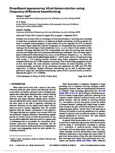
F ( W, Q ) @ H ( y ) = E ln p y ( y ) = E{ln J } + H ( x ) (4) where p y (y) is the complex domain pdf of the outputs y and J represents the Jacobian. Following [6] a non-linear function for each frequency bin should be implemented. In order to reduce the computational cost, we exploit an approximate scheme, using only a global adaptive function for all the frequencies. The overall system is reported in Figure 1, where the presence of a single non-linear function is clearly shown. 3. Complex spline non-linear function
and fractional parts using the floor operator . , finally we get
i = z ;
u = z −i
(8)
In matrix form the output for the k-th spline span, can be expressed as
(
)
yi = f i u , Q iu = Tu ⋅ M ⋅ Q iu
(9)
where: Tu = u 3
u2
1
u
−1 3 −3 1 3 −6 3 M= 6 − 3 0 3 4 1 1
(10) 1 0 0 0
(11)
with 0 ≤ u < 1 and M is the coefficient matrix of the Bspline version of [3], as in [2]. In the complex domain, we use two distinct real-valued spline functions [4], one for the real part and one for the imaginary part. Therefore equation (9) can be redefined as:
(
)
(
)
yi = hi, R u iR , Q iuiR + j ⋅ hi, I u iI , Q iuiI = = TuR ⋅ M ⋅ Qiu + j ⋅ TuI ⋅ M ⋅ Qiu iR
For a better understanding, let’s briefly introduce the realvalued case. The real spline activation functions (see [3]) are smooth parametric curves, divided in multiple tracts (spans) each controlled by four control points. Let f(x) be the non-linear function to reproduce, then the spline activation function can be expressed as:
iI
where yi is the complex output of the function and j denotes the imaginary unit. In order to ensure the monotonously increasing characteristic, we must impose the constraint: Q1 < Q2 < ...< QN , for both the real and imaginary parts.
N −3
y = f ( x ) = C fi (u , Q i )
(12)
4. Adaptation rule
(5)
i =1
i.e. as a composition of (N-2) spans fi ( u ) i=1,…,N -3 (where N is the total number of the control points Qi i=1,…,N) each depending from a local variable u ∈ [0,1) and controlled by four Qi = {Qi , Qi +1 , Qi +2 , Qi+3 } control points. The two parameters i, u can be derived by an internal variable z z=
x N −1 + ∆x 2
1 z = z N − 3
(6) if z < 1
if 1 ≤ z ≤ N − 3
(7)
if z > N − 3
where ∆ x is the fixed distance between two adjacent control points; the constraints imposed by equation (7) are necessary to keep the input within the active region that encloses the control points. Separating z into the integer
Following the information theoretic approach of eqns.(4), a rule for the adaptation of both the un-mixing matrix and the spline control points can be derived. Defining the joint entropy for a complex variable H(y) as: H ( y ) = − ∫ p y ( y R , y I )ln ( p y ( y R , y I ) )dy R dy I .
(13)
we can derive the adaptation rule for the weights W in the complex domain as [5]
{
−1
∆ Wk = µ WkH−1 + h( u) x H
}
(14)
where the suffix H denotes the matrix Hermitian. In order to derive the adaptation rule for the control points, the cost function to be maximized can be redefined as: F ( W , Q R, Q I ) @ H (y ) .
(15)
where the arrays QR and QI indicate respectively the real and imaginary parts of all the B-spline control points,
Considering the activation function defined in eq. (12), the j-th element of h(u), assumes the form: ∂y′jR ( u jR ) ∂y′jI ( u jI ) 1 1 h j (u j ) = +j = y′jR ( u jR ) ∂ u jR y′jI ( u jI ) ∂ u jI (16) && && 1 Tu jR MQiu jR 1 Tu jI MQiu jI = + j & MQ & MQ ∆u jR T ∆u jI T u jR iu uI iu jR
jI
where for the sake of simplicity we assume ∆u jR equal to ∆u jI (as in practical cases). In order to adapt the control points of the activation functions, first it is possible to show that the maximization of the functional (15) is equivalent to the maximization of the following quantity:
∑ ln ( y ′ ) +∑ ln ( y ′ ) + ln (det W% ) N
N
jR
j =1
j =1
(17)
jI
% is a suitable matrix depending of the un-mixing where W matrix W which does no depend on the control points. Then, starting from this, it is possible to demonstrate that the adaptation rule for the control points of the real part function can be expressed as:
∆QiujR + m
N N ∂ ∑ ln ( y′kR ) + ∑ ln ( ykI′ ) k =1 k =1 ∂ ln y′jR ∝ = = ∂Qiu + m ∂Qiu + m
( )
jR
=
∆u jR 1 ∂y′jR = & y′jR ∂Qiu +m Tu jR MQiu jR
(
& MQ ∂ T u jR iu jR
∆u jR∂Qiu
jR
jR
)=
+m
(18)
jR
& M T u jR m
& MQ T u jR iu
6. References
jR
A similar expression can be derived for the control points of the imaginary part function, so we can write the final adaptation rule as: ∆ Qiu jR + m = η ∆ Qiu
jI
+m
=η
&u Mm T jR
& MQ T u jR iu & M T u jI m
jR
.
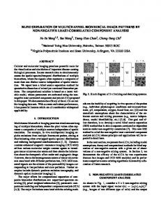
where we consider a 2-channel MBD problem, this allows to adapt only 4 real spline functions (1 complex function per channel, 2 real functions each). The experiment consists of the blind deconvolution of two signals obtained by mixing two speech signals with a minimum phase 2x2 filter matrix. Both the classical algorithm (without adaptive functions) and the proposed adaptive scheme has been implemented and tested on the signals. For the new architecture, the FFT output has been scaled in order to fit the selected input range of the real spline functions (-3, +3). The estimated probability density functions of the input signals (real and imaginary parts) are reported in the first row of Figure 2. The second row of the same figure reports instead the shapes of the corresponding adaptive functions after adaptation, compared with the static tanh function. The adaptive capability of the proposed method is well evident. This is confirmed also by the performance in frequency, obtained activating only a channel at a time as in [6]. Fig. 3 reports such results for the spline-based algorithm (left column) and for the case of static (non-adaptive) functions (right column). Figure 4, instead, reports the evolution of the Signal-toNoise (S/N) ratio during adaptation. The dark gray lines represent the evolution of S/N (in the two channels) for the adaptive spline case, while the light gray lines are relative to the static case. Again the gain in performance of the proposed method can be appreciated.
(19)
& MQ T u jI iujI
where the term η represents the constant adaptation rate for the B-splines control points. For the sake of brevity, the two derivations are not reported here. 5. Experimental results In order to test the performance of the proposed algorithm several experiments has been carried out. Due to the space limitation we report only one experiment relative to a minimum phase convolutive mixing. As stated before, in order to reduce the computational cost, the proposed architecture uses an approximate scheme using only one complex-valued adaptive function for all the frequencies (Figure 1). In the experiment we report,
[1] A.J.Bell, T.J.Seinowski, ”An information-maximization approach to blind separation and blind deconvolution”, Neural Computation, vol.7, pp.1129-1159, 1995. [2] A. Pierani, F. Piazza, M. Solazzi, A. Uncini, “Low Complexity Adaptive Non-Linear Function for Blind Signal Separation”, Proc. of IEEE IJCNN2000, Como , Italy, 2427 July 2000. [3] S. Guarnieri, F. Piazza and A. Uncini, “Multilayer Feedforward Networks with Adaptive Spline Activation Function”, IEEE Trans. on Neural Network, Vol. 10, No. 3, pp.672-683, May 1999. [4] A.Uncini, L.Vecci, P.Campolucci, F.Piazza, “Complexvalued neural networks with adaptive splinae activation function”, IEEE Trans. on Signal Processing, vol.47 N° 2 Feb. 1999. [5] T.W. Lee, A.Bell, R. H. Lambert, “Blind separation of delayed and convolved sources”, In Advances in Neural Information Proc. Systems 9, pp. 758-764, MIT Press 1997 [6] P.Smaragdis, “Blind separation of convolved mixtures in the frequency domain” in Proc. International workshop on Indipendence & Artificial Neural Networks, Tenerife, Spain, February, 9-10 1998.
x(t)
X(1)
x(t-1)
X(2)
W1
U(1)
y(t) y(t-1)
W2 f ()
FFT
IFFT
U(2) x(t-N+1)
X(N)
WN
y(t-N+1) U(N)
Figure 1: The proposed frequency domain architecture using one adaptive flexible B-spline activation function.
Figure 2: Input signal pdf’s and the corresponding adapted spline functions.
output 1
output 1
40
40 u1/s1 u1/s2
0 -20
0 -20
-40 10
u1/s1 u1/s2
20
dB
dB
20
-40 0
10
1
10
2
10
3
10
4
10
0
10
1
output 2 40
2
10 output 2
10
3
10
4
40 u2/s2
u2/s2
20
20
u2/s1
0
dB
dB
u2/s1
-20
-20
-40 10
0
-40 0
10
1
10
2
frequency (Hz)
10
3
10
4
10
0
10
1
10
2
10
3
frequency (Hz)
Figure 3: Performance in frequency domain: (left) using adaptive functions; (right) fixed tanh functions.
Figure 4: SNR during the learning phase: (left)using adaptive functions; (right) fixed tanh functions.
10
4