Accepted Manuscript Title: Blind Deconvolution Using Maximum A Posteriori (MAP) Estimation With Directional Edge Based Priori Author: Rani Aishwarya SN Dr. Vivek Maik PII: DOI: Reference:
S0030-4026(17)30301-7 http://dx.doi.org/doi:10.1016/j.ijleo.2017.03.041 IJLEO 58964
To appear in: Received date: Accepted date:
21-2-2017 13-3-2017
Please cite this article as: Rani Aishwarya SN, Dr. Vivek Maik, Blind Deconvolution Using Maximum A Posteriori (MAP) Estimation With Directional Edge Based Priori, (2017), http://dx.doi.org/10.1016/j.ijleo.2017.03.041 This is a PDF file of an unedited manuscript that has been accepted for publication. As a service to our customers we are providing this early version of the manuscript. The manuscript will undergo copyediting, typesetting, and review of the resulting proof before it is published in its final form. Please note that during the production process errors may be discovered which could affect the content, and all legal disclaimers that apply to the journal pertain.
Rani Aishwarya S N1 , Dr.Vivek Maik2 School of Electronics and Communication
cr
Oxford College of Engineering, Bengaluru, India 560068
us
a The
ip t
Blind Deconvolution Using Maximum A Posteriori (MAP) Estimation With Directional Edge Based Priori.
Abstract
an
Image Inverse problem or ill-posed problem has been tackled by various researchers in a number of ways. The number of unknown parameters as well as the properties of the parameters makes the problem very challenging. Major-
M
ity of the research has been focused on using image properties and any prior knowledge of the bwr or degradation phenomenon. The whole process can be classified in to three categories: (i) Blind methods (ii) Semi blind methods (iii)
d
Non blind methods. The proposed work in this paper is based on semi blind
te
method where partial prior in the form of directional edges were used. The Bayesian class of methods using Maximum A Posteriori (MAP) estimates were
Ac ce p
proven very successful and used here. The main contribution of the proposed method involves (i) Alternating minimization step for PSF (blur) and shape image (ii) Regularization based on adaptive directional gradients (iii) Non-local minima using edge features. The experimental result shows that the proposed algorithm is better than other enriching methods. Keywords: Blind Deconvolution, Directional Priors, Augmented Lagrangian Methods, PSF Estimation, Inverse Filtering.
I The authors are with Department of Electronics and Communication, The Visvesvaraya technological University, Belgaum, Karnataka 560018. Email address:
[email protected],
[email protected] (Rani Aishwarya S N1 , Dr.Vivek Maik2 )
Preprint submitted to Journal of LATEX Templates
March 17, 2017
Page 1 of 30
1. Introduction
ip t
The formation of image in cameras happens very similar to human eye vision. The reaction of the camera, sensors to the visible light depends on lot of optical parameters includes focal length, exposure, lens curvature, etc. Other external
factors such as environmental background, angle of camera, movement of object
cr
5
play a pivotal role in image formation. Also for many novoice to advanced
us
photographers capturing an ideal settings image becomes challenging because of the sheer number of intrinsic and extrinsic parameters. This is also the same reason that many a times the captured image suffers from various anomaly or
an
distortion such as noise, blur, low contrast etc.
te
d
M
10
Fig 1. Block diagram representation of image formation. As shown in the Fig.1. once the image is recorded at the sensor level the
Ac ce p
connection of image with optical methods becomes impossible. This is where
15
the use of digital algorithms becomes necessary. The digital algorithms work with images representing them as 2D matrices and using mathematical technique to digitally correct them. Several such algorithm methods have been developed in the past for removing noise in images, degradation, contrast enhancement, image reconstruction etc.
20
In our work we focus on the image restoration part. Image restoration
methods are also known as Deconvolution methods. This is because the blur is mined with the image as convolution sum. Therefore the removal of blur from the image becomes the reverse process of convolution known commonly as Deconvolution as shown in the Table I. The latter problem of deconvolution is very
25
challenging as it involves the inverse of blur operator H. The degraded image y 2
Page 2 of 30
Table 1: Description of convolution and deconvolution.
Deconvolution
y = Hx
y = Hx
Find y
Find x
cr
ip t
Convolution
is the digital image obtained from detective cameras settings which needs to be
us
restored. In most of the restored algorithm it often becomes necessary to find the blur ”H” and the sharp image ”x” is restored. Therefore we can see that for y = Hx we have two unknown quantities in the form of H and known quantity in the form of y. The above class of problem comes under the category of ill-
an
30
posed problem. The well-posed problem is when number of unknown quantities
M
is equal to number of known quantities.
The solution to ill-posed problem is not often straight forward and requires the use of numerical optimization techniques. In our paper we adopt a Bayesian class of numerical estimates with directional regularization. The main contri-
d
35
bution and novelty of the proposed method is described in the coming sections.
te
The performance of the given techniques is compared with other existing meth-
Ac ce p
ods and the proposed algorithm gives better result than their counterparts. 1.1. Blur Phenomenon in Images
40
The image blur can occur in number of ways. Some of the common causes
of blur include motion, defocus, camera shake, lens aberration, optical defects, etc. The blur in images is often mathematically represented using point spread function (PSF). Removing the blur or PSF from image pose a very important problem statement in the field of Image processing. Removal of blur from
45
an image is the same as estimating the PSF which is usually in the form of a smaller matrix or kernel of size anywhere between 3x3 to 11x11. The usual methods for estimating PSF adopt some form of prior information which is then evolved using a iterative process until the desired PSF is achieved. The initial PSF estimate usually takes image features like edge structures as shown in Fig.2
3
Page 3 of 30
us
cr
ip t
50
an
Fig 2. The image represents the nature of blur and without blurness.
In the above image the dotted line represent the edge structure without blur and slanted line represent the edges after blurring. The comparative measure
M
55
between blurred and slant edge can be a good approximation for the PSF initial estimate. Other methods usually take in the assumption the distributive
d
property of the blur. Most common distributive function used in the Gaussian
60
te
distributive function. The other parametric and statistical models have also been used to model the initial PSF estimate. In our work we will be using the Gaussian distribution function as the initial PSF estimate value and later incor-
Ac ce p
porate the feature based updates to it iteratively. The proposed algorithm in addition to taking edge features also incorporates additional constraints in the form of orientation of the edges. The adaptive behaviour in PSF estimate ac-
65
cordingly to the orientation of the edges makes it more effective in our approach. Some other PSF or blur kernel estimation methods include use of natural image statistics [3,4,5], joint posterior probability function [6,7], alpha matte for blur kernel [8,9], use of Shock filter [10], gradient threshold [11], kernel refinement step [12] are some of the entity literature for the blur kernel or PSF estimation.
70
2. Related Work Many of the deconvolution methods for the linear inverse problem or ill posed problems make use of converse and non-local regularizers [10,11]. Other set of 4
Page 4 of 30
methods used iterative Shrinkage or thresholding as two step methods in form of TWIST, FISTA and accelerated spaRSA variants. These methods proved to be faster and effective for deconvolution problem. The above problem has also
minφ(β)β
St. ||Hx3 − y||22
(1)
cr
been viewed as langrangian constrained optimization problem as,
ip t
75
us
The solution to above constrained optimization problem is either 0 or the minima [12, 13]. The above constraint problem has also been tackled with wavelet basis [14], though Fourier is the more common approach. The iterative shrinkage or method [15] rely on more general minimization step given by
an
80
1 minx ||Ax − y||22 + λC(x) 2
(2)
M
where A = Hβ. The various derivatives of iterative shrinkage include majorization maximization algorithm [17]. Also over the past decade a lot of works has been carried out for combining edge or image detail presenting strategy [19, 20].
with deblurring. Blur Phenomenon during aerial or satellite imagery has also
te
85
d
These algorithms mainly try to overcome the ringing artifacts usually associated
been studied under atmospheric turbulence and makes use of the turbulence
Ac ce p
properties for blur kernel estimation and recovery of original image [20]. In [22] they have adopted polynomial approximation in the form of Bezout’s identity of coprime polynomials. The noise tolerance of the above algorithms is still ques-
90
tionable. Many algorithms though good with deblurring are often sensitive to noise. For noisy cases direct algorithms work better than indirect algorithms. Approaches using Auto regressive (AR) models are proven effective for noisy cases [24]. In this work we focus on the blur rather than noise, so this area is not explored in detail. Large number of researchers has worked with Total Vari-
95
ational (TV) regularizer to better work with image details [25, 26]. Different variations of TV algorithm were also developed on the basis of how the edges are presented [27, 28, and 29]. The TV regularization success mainly depended on the good image prior. In [33] they have adopted a variational Bayesian approach with a mixture of Gaussian image prior for modelling natural image 5
Page 5 of 30
100
statistics. The proposed paper is based on maximum a posteriori (MAP) estimation [29]. The common conception that most of the natural images have
ip t
Gaussian characteristics and blurring tend to deviate the images from the nat-
ural image characteristics. The main disadvantage of MAP stems from this fact
105
cr
that blurred image also to a certain extent exhibit Gaussian characteristics. In
[30], its been claimed that a proper estimator matters more than the shape of
us
priors. It was also shown that marginalizing the posterior with respect to latent image leads to the correct solution of the PSF or blur. Many of the MAP approaches [31] converge to the minima using adhoc steps. The proposed paper
110
an
works with MAP also but the adhoc steps are removed and replaced with image edge priors and utilize augmented lagrangian with Bregman iterations to tackle this non-convert optimization. Recently natural image statistics have been used
M
over gradients to good effect [32]. Some of the drawbacks of the MAP method include ineffective global minima or many suboptimal local minima which could lead to subsequent convergent mimics. More often the convergent solutions require tradeoff between parameters and other regularizers. To mitigate some of
d
115
te
these shortcomings of MAP the [33] propose to solve the above. (3)
Ac ce p
maxk P (k | y) = mink − 2logP (y | k)P (k)
This technique is also used in the proposed work.
3. Problem Statement of Deblurring
120
The recovery of a sharp image from a blurred and noisy image is deblurring.
Deblurring with no knowledge of the PSF (Point Spread function) amounts to blind deconvolution.
6
Page 6 of 30
ip t cr
125
Fig 3. Block Diagram Representation of the Problem Statement.
us
Many iterative and non-iterative blind deconvolution algorithms and techniques in recent times have attempted to solve this problem and have made progress, yet many aspects of blind deconvolution remains challenging. Recovery of a sharp image from a single source of observation or a single blurred
an
130
image is the SCBD (Single Channel Blind Deconvolution) which is extremely
M
ill posed. The problem can be better posed by assuming multiple sources of observation, i.e. by using multiple blurred images of the same object leading to MCBD (Multi Channel Blind Deconvolution).
Though slightly better posed than the single channel blind deconvolution,
d
135
the multi-channel problem consists of many challenging aspects. It satisfies
te
the convolution degradation model represented by the equation in (1). Many similar methods of better posing the challenging problem statement exist. For
Ac ce p
the course of this journal though MCBD is better posed the problem statement
140
is assumed to be a single channel blind deconvolution problem due to its vast scope of modifications and improvement. The Problem Statement is represented by the equation, g =h∗u+n
(4)
where, g = input blurred image. h = estimated PSF.
145
u = output sharp image. n = random noise. ∗ = convolution operation. + = addition operation.
7
Page 7 of 30
The input blurred image g represents the single channel of observation. The 150
unknown blur function or the point spread function (PSF) for this source image
ip t
is represented by h which is in convolution with the sharp image u. Hence the
sharp image u can be derived through deconvolution. The simultaneous estima-
cr
tion of the blur kernel h and the sharp image u amounts to blind deconvolution.
The random noise that is added to the model is represented by n. The PSF is assumed to be space invariant which means every point in the original image
an
moves in the manner to generate the blur.
us
155
Fig 4. Depiction of A Well-Posed Problem.
This is usually caused by linear motion blurring due to relative motion be-
M
160
tween camera and the object. This problem statement is very challenging and has been a topic for many researchers around the world. The problem statement
d
constitutes of various issues within it. Hence to solve the problem statement
165
te
as a whole each of these problems has to be considered and solved. Each and every one of these problems is challenging enough for a research thesis listed as
Ac ce p
follows:
(i) Ill posed problem. (ii) Inverse Problem.
(iii) Inverse-Ill posed Problem.
170
(iv) Blind Deconvolution Problem. Since the problem statement is complex, a perfect solution to the problem
cannot be found. Therefore the scope of improvement in existing methodologies is high.
175
(i) Ill-posed Problem: The problem statement in equation (1) satisfies all the defined criteria describing an ill-posed problem. The standard definitions for an ill-posed problem
8
Page 8 of 30
as defined by both Jacques Hadamard and Nashed are used to confirm that the problem statement is indeed an ill-posed problem. The convolution model represented in equation (1) defines the problem state-
ip t
180
ment. It does not necessarily have a solution. Further, solving the problem de-
cr
fined in the equation (1) to find the sharp image u has led to many algorithms from many researchers. The solution thus found using various techniques is not
185
us
unique. Also the solution varies with the variation in the assumption of input data or priors required to solve the problem. The priors assumed and the data observed may or may not be a closed set. The problem is also extremely ill-posed
an
with three set of unknowns h, u and n and a single known value g describing it. The problem statement is mathematically ill-posed due to an information deficit. (ii) Inverse Problem:
M
190
The conventional forward approach model is one where a set of data is observed from the models parameters. Here the data n is derived from the existing
d
model m. While a typical inverse model is one where the parameters of the model
195
te
is derived from a set of data which is given or assumed prior to the experiment. Here the parameters of the model ’m’ are derived from the data ’n’ either given
Ac ce p
or assumed in the mathematical model defining the system. Inverse problems can be categorized as either parameter estimation or design optimization problems.
200
Fig 5. Block Diagram Representation of Convolution Theorem.
9
Page 9 of 30
The problem of sharp image recovery from a blurred image is that of pa-
205
ip t
rameter estimation from the observed data. The models parameters i.e. its blur function h is derived from a set of data comprising of blurred image g which is
cr
given, along with the appropriate priors assumed. Assumption of appropriate
priors is necessary for the accurate estimation of the blur kernel. Now from the
us
parameters derived we further optimize the design to recover the sharp image u. This is a design optimization problem. The recovery of sharp image u can be 210
either simultaneous or consecutive. The estimation of the sharp image u along
an
with the blur function h is simultaneous. Whereas the recovery of u from the blur function h, after its estimation is consecutive. (iii) Inverse-Ill posed Problem:
215
M
This inverse problem is also ill-posed due to lack of necessary data. Hence the problem statement of the model represented in equation is an ill posedinverse problem.One of the various methods to estimate the blur kernel h in the
d
inverse problem is by inverse filtering.
te
g =h∗u+n
(5)
To reduce the complexity of solving this problem the random noise n in the
Ac ce p
model is assumed to be zero, i.e. consider n=0 then,
220
g =h∗u
(6)
Now solving for u gives, u = g = h and u = g/h. Hence it is deduced that estimating the accurate blur kernel is necessary for image restoration. By using inverse filtering techniques to find h-1, the sharp image u can be recovered. (iv) The Blind Deconvolution Problem: From Convolution Theorem time domain representation is, g(t) = u(t) ∗ h(t)
225
(7)
where * denotes convolution operation in Frequency Domain it changes to, G(w) = U (w) ∗ H(w)
(8)
10
Page 10 of 30
Convolution in time domain is converted to multiplication or dot product in frequency domain. Thus by applying the algorithm in frequency domain
ip t
reduces the computational complexity. Hence high resolution color images can be restored with more ease.
The recovery of the sharp image u from the convolution degradation model
cr
230
amounts to deconvolution. Mathematically convolution increases in complexity
us
with the number of elements in the operation. The number of pixels in an image determines the number of elements. Hence restoring color images with high resolution will be more complex as color images have more pixel values, set of pixel values for each RGB. By removing or replacing the convolution
an
235
operation this complexity can be removed. Converting an equation in time domain to frequency domain converts the convolution operation in time domain
M
to dot product in frequency domain.
(9)
d
G(w) = U (w) ∗ H(w)
The deconvolution problem of recovering the sharp image mathematically through deconvolution is blind as both the blur kernel h and the sharp image u
te
240
are unknown. Hence it is called a blind deconvolution problem. Solving a blind
Ac ce p
deconvolution problem is a optimization problem. Optimization of a solution to the problem can be achieved through numerous optimization techniques. Some of them are convex optimization and constraint optimization techniques that
245
are the most used in image processing. The constrained optimization is used for the mathematical model used in this thesis. Hence constrained optimization technique is adapted in the algorithm. A constrained or a constraint problem where the objective function which
has to be solved is subject to constraints a constraint function which describes
250
the constraints to which the objective function is being subject to. Hence a constraint problem should give a solution to its objective function such that it is within the limits of the constraints that it is limited to.
11
Page 11 of 30
H step
Min u
Min h
Minimization w.r.t u
Minimization w.r.t h
FT w.r.t edge
FT w.r.t image derivatives
FT of H(g)
FT of U(g)
FT of H(g) ∗ U (g)
FT of U (g) ∗ Fdx
us
an
4. Proposed Methodology 255
cr
U step
ip t
Table 2: Performance comparision of delta.
The proposed method is implemented entirely in the frequency domain. The minimization algorithm is carried out as shown in Table 2.
M
(i) U-step Minimization:
The Fourier transform for u- step is with respect to the edge taper function to reduce the border effects. The transpose of the blur kernel H and the input image g is converted to frequency domain. This is multiplied with the Fourier
d
260
te
transformed edge taper function Eg .
Ac ce p
Ht (w) = g(w) ∗ Eg (w)
(10)
Here Ht (w),g(w) and Eg (w) represents the blur function and the edge taper function in the frequency domain. Similarly, the Fourier transform for h- step is calculated with respect to the image derivatives. The transpose of the image
265
function is converted to frequency domain. This is multiplied with the derivatives of the image given by F (dx) and F (dy). Ut = F (dx)g(w) ∗ F (dy)g(w)
(11)
where Ut g(w) and F (dx)g(w) ∗ F (dy)g(w) represent the image function and the image derivatives in the frequency domain. The Maximum A Posteriori (MAP) estimate of the problem statement is 270
the equivalent of the minimization of the equation below, Maximization of the
12
Page 12 of 30
posterior estimate is equivalent to the minimization of its negative algorithm,
=
−log(P (u, h|g)) + const,
=
−γ/2||(u ∗ h − g)2 || + Q(u) + R(h) + const
(12)
cr
L(u, h)
ip t
i. e.,
where Q(u) = −logP (u) and R(h) = −logP (h) are the regularizes Sepa-
275
us
rating the equation for the u-step and the h-step, by minimizing the function L with respect to either u or h while keeping the others constant. Thus two different minimization problems are derived one for the u - step and other for
an
the h - step from the single existing minimization problem.
The minimization of the Maximum A Posteriori (MAP) estimate gives negative algorithm for the u step,
M
γ minu ||(hu − g)2 || + φ(Dx u, Dy u) 2
(13)
s.t,
d
280
te
Vx = Dxu ,Vy = Dyu
γ minu ||(hu − g)2 || + φ(Vx , Vy ) 2
(14)
Ac ce p
The equation gives the minimization problem for the u - step. Similarly the minimization of the Maximum A Posteriori (MAP) estimate
gives negative algorithm for the h step. Here to separate the data term and
285
regularizer term we substitute V h = h. Hence we derive the objective fuction
below,
γ minh ||(Uu − g)2 || + R(Vx ) 2
(15)
subject to constraints,h = Vh Now the minimization problem derived for both the u-step and h-step are constraint optimization problems hence to solve for the numerical value of u
290
and h an Augmented Lagrangian Method (ALM) is employed.
13
Page 13 of 30
Applying ALM the constrained function in equation is converted to the
ip t
295
unconstraint function below,
cr
γ = minu ||(hu − g)2 || + φ(Vx , Vy ) 2 α α ||(Dx u − Vx − Ax )2 || + ||(Dy u − Vy − Ay )2 || (16) + 2 2
us
Lu (U, Vx , Vy )
(ii) H - step Minimization :
Similarly by applying ALM the constrained minimization function in equa-
Lh (h, Vh ) =
γ β ||(uh − g)2 || + R(vh ) + ||(h − Vy − ah )2 || 2 2
(17)
The Proposed algorithm uses K1 norm regularization due to its sparse na-
M
300
an
tions results in the unconstrained functional given by the equation below,
ture. Here the regularizers used are the L1 norm of the image derivatives either
edges.
d
Laplacian distribution of image derivatives or heavy tailed gradient from tapered
derivatives which is directionally separable is given by,
Ac ce p
305
te
The L1 norm of the image derivatives using Laplacian distribution of image
Q(u) =
X [Dx u] + [Dy u]i hu
(18)
t
Similarly the L1 norm of the image derivatives using Heavy tailed gradients
gives,
Q(u) = φ(Dx u, Dy u) =
X ([Dx u]2i + [Dy u]2i )2
(19)
t
where DX and DY are partial derivative operators and 0 < p < 1. To achieve a sparse blur kernel the L1 norm regularization is employed to the
310
image gradients using a Laplace distribution and isotropic image gradients are used. For applying the regularizer to the blur kernel the Laplace distribution on the positive kernel values is used in order to achieve sparsity and to convert the negative values to zero.
14
Page 14 of 30
Table 3: Optimization for u - step and h - step.
Minimization w.r.t h
g-blurred image
g-blurred image
Image derivatives
Image derivatives
H estimates
U estimates
Lp-norm priors
Lp-norm priors
Guassian priors
Guassian priors
X t
cr
us
φ(hi )
(20)
h if h ≥ 0; i i φ(hi ) = ∞ if h < 0. i
M
315
an
This results in the following regularizer R. R(h) =
ip t
Minimization w.r.t u
Now the regularizer in terms of Isotropic image gradient is given by, Xp
([Dx u]i 2 + [DY u]i 2 )
d
Q(u) =
(21)
te
t
where DX and DY are partial derivative operators and 0 < p < 1. The iterative alternative minimization with respect to u and h is continued
Ac ce p
until the maximum number of iterations is reached or the convergence point
320
is reached. The table II shows the different parameters required to find the numerical value of h and u estimates. The numerical value of the estimated PSF h and the sharp image u is updated at the end of each iterative step. Hence at the end of the iterative optimization procedure the accurate estimated PSF h and the sharp image u is obtained.
325
The Mean Squared Error of the estimated blur is calculated by, n
M SE =
1X ˆ (hi − hi )2 n i−1
(22)
ˆ is the estimated PSF and h is the actual PSF This is implemented in Here h ˆ the algorithm to calculate its accuracy. Due to simultaneous recovery both h and u the estimated PSF and the sharp image u are obtained. 15
Page 15 of 30
5. Existing Alternating Minimization Existing methodology uses alternating minimization with maximum A pos-
ip t
330
terior estimation. Numerous parametric methods for estimating a variety of
blurs have been proposed. Unfortunately real PSFs cannot be determined by
cr
a parametric model. It has been seen that Bayesian methods for PSF estima-
tion provide better blur estimates. Using Bayesian paradigm in a probabilistic model for simultaneous recovery of sharp image and PSF can be devised using
us
335
a MAP (Maximum A Posteriori) model. The priori information of the model can be used to estimate its parameters using the Bayes theorem. The Bayesian
an
inference with respect to the prior information of the image and the blur kernels are given in the equation, which gives the (MAP) estimate. Essentially MAP is a probabilistic model used to convert the problem statement to be solvable mathematically. The problem statement given by,
M
340
d
g =h∗u+n
(23)
te
Applying the MAP probabilistic model changes the problem statement to a mathematically solvable equation,
Ac ce p
M AP (u, h)
345
=
P (u, h|g) ∗ P (g|u, h)P (u, h)
=
P (g|u, h)P (u)P (h)
(24)
where,
P (u, h|g) = exp(2 ∗ k(u ∗ h − g)2k)
(25)
Here P (u, h|g) is the Gaussian noise distribution and P (u) and P (h) are the
prior distributions of the latent image and blur kernel, respectively. Maximization of the posteriorP (u, h | g) is equivalent to the minimization of its negative algorithm, i. e., L(u, h)
=
−log(P (u, h|g) + const,
=
2k(u ∗ h − g)2k + Q(u) + R(h) + const (26) 16
Page 16 of 30
ip t cr us an
M
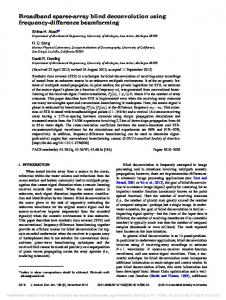
Fig 6. The Graph shows Minima of a Function and the Block Diagram shows Representation of Alternating Minimization Algorithm. where Q(u) = −logP (u) and R(h) = −logP (h) can be regarded as regularizers
d
350
te
that steer the optimization to the right solution. Here a prior is assumed only on u which allows few non-zero coefficients of some linear or nonlinear image
Ac ce p
transform. This Sparse Priors is also a straight forward approach for solving each constrained problem at every iteration step of the alternating minimization
355
algorithm. Where each constrained problem is converted to an unconstrained problem by variable splitting. The minimum of a real-valued function f(x) can be found by a method minimum optimization. It is a technique of estimating the absolute or the global minima of a function. It is shown that from the previous MAP estimate section we have derived that the problem statement is
360
converted into a mathematically solvable minimization problem. Hence finding the minimum of the function in equation and calculating its numerical value solves our problem statement. Minimum Optimization locates the global minima of a function. In order to find the numerical solution constraint optimization method is employed. Since the minimization problem in equation is a constraint
365
function, constraint optimization is best suited. By keeping h value constant 17
Page 17 of 30
and deducing for u in order to find the numerical value of the minimization
γ minu ||(hu − g)2 || + φ(Dx u, Dy u) 2
(27)
(28)
cr
vx = Dx u, vy , Dy u
ip t
problem equation is converted to,
Here the above equation referred to as objective function which has to be solved to derive the numerical value. While Objective function denotes the con-
us
370
straints that the objective function subject to but also means that the objective function has to be solved in such a way that it adheres to the limitations set by
an
the constraints that it has been subject to. Hence this is also called a constraint function. Together the objective function and the constraint function form the 375
constraint optimization problem. Hence the Augmented Lagrangian Method is
M
employed in the mathematical model to solve the above constraint optimization problem. For the superior restoration of the images an iterative algorithm for simultaneous estimation of accurate blur kernels and deblurred image which al-
image u is used. This is called the alternating minimization algorithm, as seen
te
380
d
ternately optimizes with respect to image and blur to estimate PSF h and final
Ac ce p
in its block diagram representation in fig.6. 5.1. Lp Norm Regularization Lp Norm is the most widespread regularization technique used in image
processing. Where Lp priors are introduced into a function to regularize it is
385
independent of the data. The Regularization term is independent of the data. Hence even as the complexity of the function increases the regularization term experiences no variance. While complex higher order functions, the function itself varies with increasing order then reach a solution becomes mathematically infeasible. In order to avoid this situation a regularizer term is added to the
390
function. The emphasis on the regularizer term reduces the variance of the function but it may increase its bias. Regularization balances not having too much error and keeping small parameter values. By adding regularization function the model does not choose 18
Page 18 of 30
extremely large parameter values necessary to reduce (Mean Square Error) MSE. 395
Unregularized functions become complex functions with extreme values of order
ip t
of the polynomials. While a regularized function remains a simple function even for high order polynomials. The regularization techniques mostly employed for
cr
inverse problems are L1, L2. The L1 norm of regularization is also known as
lasso. It tends to generate sparser solutions. Hence it is generally preferred in regularization. The L2 norm is also known as a quadratic regularizer. The data
us
400
points in a quadratic regularizer are more angular. Therefore the solutions are not sparse. Due to the sparse nature of its solutions the L1 norm is preferred
an
in this algorithm. 5.2. Bregman Iterations
Split Bregman Iterations is a method to solve hard optimization problems.
M
405
According to Bregman iterations by finding a feasible solution to a function it can be optimized. The convergence function in Bregman iterations is very
d
helpful in solving the problem. Therefore Bregman iterations are used along
410
algorithm.
te
with the Augmented Lagrangian Method to solve the objective function in this
Ac ce p
6. Experimental Results
The Proposed Method is implemented in Matlab. The resulting Matlab code
is executed for results. The results from the proposed method are compared with the results of the existing methodology and various existing blind deconvolution
415
algorithms. For numerical assessment of performance of the proposed method the results from the proposed method, existing method and various other existing blind deconvolution algorithms are tested for their PSNR (Peak Signal to Noise Ratio) to calculate maximum signal strength. Similarly to find the method with least error the MSE (Mean Squared Error) of the different meth-
420
ods are found. The MSE of different methods are compared and plotted in a graph. From this experiment it is concluded that the proposed method gives more accurate results in deblurring blurred images. 19
Page 19 of 30
6.1. Performance of Proposed Method
425
ip t
The performance of the proposed method is measured using: (i) MSE (Mean Squared Error).
cr
(ii) PSNR( Peak Signal to Noise Ratio).
(i) MSE:
430
us
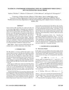
The method of using directional priors for edge prediction and preserving in the blind deconvolution algorithm using is alternating Maximum A Posteriori estimation is implemented using Matlab. This method is applied to the test
Fig 7. Experimental results generated for Lena colour and Greyscale image.
Ac ce p
435
te
d
M
an
data set of Levin et al [11]. The data set consists of four images.
Fig 8. Experimental results generated for Mandril color image. Ground truth PSFs are applied to each of the images to give a total of 32
440
test images. The MSE (Mean Square Error) of estimated blur kernel for each of the 32 examples is calculated. This is compared with the MSE of estimated blur kernels of other blind deconvolution algorithms such as alternating MAP method [1], Fergus et al.[8] , Xu and Jia [3]. The MSE of the blur kernels of
20
Page 20 of 30
various methods are plotted. Here lower MSE values of our method show better performance. Using correct directional priors lead to more accurate estimation of the PSF.
M SE = 1/n
n X
(hˆi − hi )2
i=1
450
us
ˆ is the estimated PSF h is the actual PSF. Where , h
(29)
cr
The Mean Squared Error of the estimated blur is calculated.
ip t
445
(ii) PSNR:
an
The edge detection filters of the form shown are employed in the existing algorithm using second order methods. The gradient operators are applied in
M
the form of their derivatives to estimate the first image derivatives. This gives the rate of change of intensity of first derivatives of the image also the kernels are padded with zeroes to equate the size of the image.
Ac ce p
te
d
455
Fig 9. Experimental results generated for cameraman image.
460
Fig 10. Experimental results generated for pirate image. 21
Page 21 of 30
The final deblurred image of the blurred standard test images using this pro-
ip t
posed method is compared with the deblurred images of other blind deconvolu-
tion algorithms. Edge detection leads to improved quality of restored images. The comparison of deblurred results using the proposed method and also using
cr
465
other blind deconvolution algorithms is shown for numerous test images in fig-
us
ures titled experimental results. The PSNR (Peak Signal to Noise Ratio) of the five standard test images in the data set are tabulated below. The Peak Signal to Noise Ratio of the estimated blur is calculated.
M
an
470
d
The test data set of Levin et al. [11] which is used. The four images along with
Ac ce p
te
eight ground truth PSFs give a total of 32 test images.
475
Experimental Results showing the MSE of estimated blur kernels (Lower
values means better performance) in the first 16 of the 32 examples of test images using different blind deconvolution algorithms. The x-axis shows the image
480
index and the y-axis shows MSE.
22
Page 22 of 30
Table 4: PSNR RESULTS FOR FIVE STANDARD TEST IMAGES ARE TABULATED.
Image Name
Blind
Deconvolution
Existing Method
Proposed
ip t
Sl.No
Algorithm
Method
Pirate.tif
18.9524
21.9044
22.1221
2
Cameraman.tif
17.7726
20.0398
20.7299
3
Mandrilcolor.tif
19.6267
20.5468
20.7974
4
Mandrilgray.tif
18.9498
21.3267
21.6451
5
Womanblonde.tif
18.1585
22.7255
22.8080
d
M
an
us
cr
1
Experimental Results showing the MSE of estimated blur kernels (Lower values means better performance) in the next 16 of the 32 examples of test
te
485
images using different blind deconvolution algorithms. The x-axis shows the
Ac ce p
image index and the y-axis shows MSE. P SN R = 20.log10 (M AXi ) − 10.log10 (M SE)
(30)
where,
(M AXi ) is the maximum possible pixel value of the image.
490
(M SE) is the mean squared Error of the output image. The table shows the PSNR values using different blind deconvolution algorithms.
7. APPLICATIONS The proposed method of blind deconvolution can be implemented in various 495
fields involving image processing. For example in astronomy, medical images, 23
Page 23 of 30
military, entertainment, mobile phone industry, etc. In all these fields the core application related to image procesing can be classified as a method image de-
an
us
cr
ip t
blurring.
M
500
Ac ce p
te
d
Fig 11. Application in Image Enhancement
Fig 12. Application in Image Restoration and tested in some applications
505
and these are shown in the figures here. Popular applications for the blind deconvolution algorithm include image restoration, image enhancement, image deblurring, image sharpening, applications in astronomical images and medical images.
510
24
Page 24 of 30
ip t
8. CONCLUSIONS
The inherent properties of a three dimensional view is captured in the edges
515
cr
of a two dimensional image. Hence better defined edges give a clearer im-
age. Using correct directional priors improves the existing blind deconvolution
us
algorithm using alternating Maximum A Posteriori estimation. The proposed method shows improved deblurring results compared to the existing blind deconvolution algorithms. Assuming correct directional priors is the key to improving
improved.
M
520
an
accurate PSF estimation. Hence Image restoration or deblurring can be greatly
References
[1] Filip Sroubek, Member, IEEE, and Peyman Milanfar, Fellow, IEEE ”Ro-
d
bust Multichannel Blind Deconvolution via Fast Alternating Minimiza-
525
te
tion”, IEEE Transactions on Image Processing, Vol. 21, No. 4, April 2012. [2] Jan Kotera, Filip Sroubek, and Peyman Milanfar, ”Blind Deconvolution
Ac ce p
Using Alternating Maximum a Posteriori Estimation with Heavy-Tailed Priors” , Institue of Information Theory and Automation, Academy of Sciences of the Czech Republic, Prague, Czech Republic, University of California Santa Cruz, Electrical Engineering Department, Santa Cruz CA 95064
530
USA.
[3] Xu, L., Jia,, Two-phase kernel estimation for robust motion deblurring Daniilidis, K., Maragos, P., Paragios, N. (eds.) ECCV 2010, Part I. LNCS, vol. 6311, pp. 157170. Springer, Heidelberg (2010).
[4] Joshi, N., Szeliski, R., Kriegman, D.J., PSF estimation using sharp edge 535
prediction., Proc. IEEE Conference on Computer Vision and Pattern Recognition CVPR 2008, June 2328, pp. 18 (2008).
25
Page 25 of 30
[5] R. Molina, J. Mateos, and A. K. Katsaggelos, Blind deconvolution using a variational approach to parameter, image, and blur estimation, IEEE
540
ip t
Trans. On Image Process., vol. 15, no. 12, pp 3715-3727, Dec. 2006.
[6] Xu, L., Jia,, Two-phase kernel estimation for robust motion deblurring
vol. 6311, pp. 157170. Springer, Heidelberg (2010).
cr
Daniilidis, K., Maragos, P., Paragios, N. (eds.) ECCV 2010, Part I. LNCS,
us
[7] Y.- L. You and M. Kaveh, A regularization approach to joint blur identification and image restoration, IEEE Trans. Image Process., vol. 5, no. 3, pp. 416428,1996.
an
545
[8] Fergus, R., Singh, B., Hertzmann, A., Roweis, S.T., Freeman, Removing camera shake from a single photograph., SIGGRAPH 2006: ACM SIG-
M
GRAPH 2006 Papers, pp. 787794. ACM, New York (2006). [9] G. Chantas, N. P. Galatsanos, R. Molina, A. K. Katsaggelos, Variational Bayesian image restoration with a product of spatially weighted total vari-
d
550
Feb. 2010.
te
ation image priors, IEEE Trans. Image Process., vol. 19, no. 2, pp. 351-362,
Ac ce p
[10] Money JH, Kang SH (2008) Total variation minimizing blind deconvolution with shock filter reference. Image Vis Comput 26:302314
555
[11] Levin, A., Weiss, Y., Durand, F., Freeman, W.T., Understanding blind deconvolution algorithms, IEEE Transactions on Pattern Analysis and Machine Intelligence 33(12), 23542367 (2011).
[12] M. Afonso, J. Bioucas-Dias, M. Figueiredo, Fast image recovery using variable splitting and constrained optimization, IEEE Trans. Image Proc., vol.
560
19, pp. 23452356, 2010. [13] Afonso, M. Bioucas-Dias, M.A.T. Figueiredo, An augmented Lagrangian approach to the constrained optimization formulation of imaging inverse problems, IEEE Trans. Image Proc., vol. 20, pp. 681695, 2011.
26
Page 26 of 30
[14] A. Beck and M. Teboulle, Fast gradient-based algorithms for constrained total variation image denoising and deblurring problems, IEEE Trans. On Image Process., vol. 18, no. 11, pp. 2419-2434, Nov. 2009.
ip t
565
[15] A. Beck and M. Teboulle, A fast iterative shrinkage thresholding algorithm
cr
for linear inverse problems, SIAM J. Imaging Sciences, vol. 2, no. 1:183202, 2009.
[16] Anat Levin, Yair Weiss, Fredo durand, William T. Freeman, Efficient
us
570
marginal likelihood optimization in blind deconvolution, in IEEE CVPR,
an
2011.
[17] J.M. Bioucas Dias, and M.A.T. Figueiredo. A new TwIST: two-step iterative shrinkage/thresholding algorithms for image restoration, IEEE Trans. Image Proc., vol.16, no.12, pp.2992-3004, 2007.
M
575
[18] R. Liu, J. Jia, Reducing boundary artifacts in image deconvolution, in IEEE
d
ICIP, 2008.
te
[19] M. Almeida, M. Figueiredo, New stopping criteria for iterative blind image deblurring based on residual whiteness measures, in IEEE Statist. Sig. Proc. Worksh., 2011, pp. 337340.
Ac ce p
580
[20] R. Molina, J. Mateos, and A. K. Katsaggelos, Blind deconvolution using a variational approach to parameter, image, and blur estimation, IEEE Trans. On Image Process., vol. 15, no. 12, pp 3715-3727,Dec. 2006.
[21] Vivek Maik, Dohee Cho, Jeongho Shin, and Joonki Paik , ”Regularized
585
Restoration Using Image Fusion for Digital Auto-Focusing” , IEEE Transactions On Circuits And Systems For Video Technology, Vol. 17, No. 10, October 2007.
[22] C. H. Fang, A New Method for Solving the polynominal generalized Bezout identity, IEEE Trans. on Circuits and systems-1:Fundamental Theory and 590
Applications, Vol. 39, No. 1, pp. 63-65, 1992.
27
Page 27 of 30
[23] Levin, A., Weiss, Y., Durand, F., Freeman, W.T., Understanding and evaluating blind deconvolution algorithms., IEEE Conference on Computer Vi-
ip t
sion and Pattern Recognition, CVPR 2009, pp. 19641971 (2009).
[24] Y. You and M. Kaveh, A regularization approach to joint blur identication and image restoration, IEEE Trans. Image Process., vol. 5, 416428, 1996.
cr
595
[25] W. Li, Q. Li, W. Gong, S. Tang, Total variation blind deconvolution em-
us
ploying split Bregman iteration, J. Vis. Comun. Image Represent., vol. 23, pp. 409417, 2012.
600
an
[26] T. Chan, S. Esedoglu, F. Park, and A. Yip, Recent developments in total variation image restoration, in Mathematical Models of Computer Vision, N. Paragios, Y. Chen, and O. Faugeras, Eds. New York: Springer Verlag,
M
2005.
[27] J. Oliveira, J. M. Bioucas-Dia, M. Figueiredo, and, Adaptive total variation
ing, vol. 89, no. 9, pp. 1683-1693, Sep. 2009.
te
605
d
image deblurring: a majorization-minimization approach, Signal Process-
[28] Babacan SD, Molina R, Katsaggelos AK ,Variational Bayesian blind de-
Ac ce p
convolution using a total variation prior. IEEE Trans Image Process 18:1226,2009
[29] Chan TF, Wong C-K ,Total variation blind deconvolution. IEEE Trans
610
Image Process 7:370375,1998.
[30] Galatsanos, N.P., Mesarovic, V.Z., Molina, R., Katsaggelos, A.K, Hierarchical Bayesian image restoration from partially known blurs., IEEE Transactions on Image Processing 9(10), 17841797 (2000).
[31] He L, Marquina A, Osher SJ, Blind deconvolution using TVregularization 615
and Bregman iteration. Int J Imaging Syst Technol 15:7483,2005. [32] M. Almeida, L. Almeida, Blind and semi-blind deblurring of natural images, IEEE Trans. Image Proc., vol. 19, pp. 3652, 2010. 28
Page 28 of 30
[33] S. Babacan, R. Molina, A. Katsaggelos, Variational Bayesian blind deconvolution using a total variation prior, IEEE Trans.Image Proc., vol.
ip t
18, pp. 1226, 2009.
an
us
cr
620
Rani Aishwarya S N is a student of Electronics and
M
Communication at The Oxford College of Engineering, Visvesvaraya Technical University (VTU) pursuing M Tech in VLSI DESIGN AND EMBEDDED SYS625
TEMS (VLSI). Currently working on Image Processing under Dr.Vivek Maik.
d
She is currently performing research on Sparse and deblurring. I have attended
Ac ce p
the IEEE.
te
many conference and submitted papers in that conference. She is a member of
630
Dr. Vivek Maik received his B tech degree in Elec-
tronics and communication at Cochin University. He received Masters and PhD in Image Processing from Chung-Ang University (CAU) Seoul, Korea, in 2010. Currently, he is serving as Associate Professor in Electronics and Communication at the University of VTU, Karnataka, India. Before starting his professor
635
carrier, he worked at the Korea Samsung Electronics as an assistant researcher. He was involved in various projects including lenses, semiconductor chips. His 29
Page 29 of 30
research interests includes Sparse representation, Image Deblurring, Super res-
Ac ce p
te
d
M
an
us
cr
ip t
olution, Reranking and many. He is guiding many PhD students.
30
Page 30 of 30