Blind Tensor-Based Identification of Memoryless Multiuser ... - eurasip

15th European Signal Processing Conference (EUSIPCO 2007), Poznan, Poland, September 3-7, 2007, copyright by EURASIP

BLIND TENSOR-BASED IDENTIFICATION OF MEMORYLESS MULTIUSER VOLTERRA CHANNELS USING SOS AND MODULATION CODES Carlos Alexandre R. FERNANDES∗, G´erard FAVIER and Jo˜ao Cesar M. MOTA I3S Laboratory, CNRS - University of Nice Sophia - Antipolis 2000 route des Lucioles, BP 121, 06903, Sophia-Antipolis Cedex, France phone: + (33) 492942701, fax: + (33) 492942898, email: {acarlos,favier}@i3s.unice.fr GTEL Laboratory - DETI, Federal University of Cear´a Campus do Pici, 60.755-640, 6007, Fortaleza, Brazil phone: + (5585) 33669467, fax: + (5585) 33669468, email: {carlosalexandre,mota}@deti.ufc.br

ABSTRACT In this paper, a channel identification technique using Second Order Statistics (SOS) is proposed for memoryless multiuser Volterra communication channels. The Parallel Factor (PARAFAC) decomposition of a third order tensor formed from spatio-temporal covariance matrices of the received signals is considered by using the Alternating Least Squares (ALS) algorithm. Modulation codes (constrained codes) are used to ensure some orthogonality constraints of the transmitted signals. That constitutes a new application of modulation codes, aiming to introduce temporal redundancy and ensure some statistical properties. Identifiability conditions for the problem under consideration are addressed and simulation results illustrate the performance of the proposed estimation method. 1. INTRODUCTION In this paper, a channel estimation technique for memoryless multiuser Volterra communication systems is proposed. The channel is modelled as a complex-valued linear-cubic Multiple-InputMultiple-Output (MIMO) Volterra filter, consisting of a generic representation of instantaneous linear-cubic polynomial mixtures. The nonlinear polynomial mixtures models have important applications in the field of telecommunications to model wireless communication links with nonlinear power amplifiers [1] and uplink channels in Radio Over Fiber (ROF) multiuser communication systems [2]. The ROF links have found a new important application with their introduction in microcellular wireless networks [3, 4]. In such systems, the uplink transmission is done from a mobile station towards a Radio Access Point, the transmitted signals being converted in optical frequencies by a laser diode and then retransmitted through optical fibers. Important nonlinear distortions are introduced by the electrical-optical (E/O) conversion [3, 4]. When the length of the optical fiber is short (few kilometers) and the radio frequency has an order of GHz, the dispersion of the fiber is negligible [5]. In this case, the nonlinear distortion arising from the E/O conversion process becomes preponderant [3, 4, 5]. Up to several Mbps, the ROF channel can be considered as a memoryless link [2, 3]. Thus, the channel is composed of a wireless link, which can be modelled as a linear instantaneous mixture, followed by electrical-optical (E/O) conversions, which can be modelled as memoryless nonlinearities [2]. Moreover, in this application, the channel nonlinearity is modelled as a third order polynomial [2, 3]. So, the overall channel corresponds to a third order memoryless multiuser Volterra system. There are few works dealing with the problem of blind source separation or/and identification of nonlinear systems in the context of multiuser communication channels. Among them, we cite [6] that proposes a blind Zero Forcing technique for Code Division Multiple Access (CDMA) systems and [7], where semi-blind and ∗C.

A. R. FERNANDES is scholarship supported by CAPES/Brazil

agency.

©2007 EURASIP

blind source separation algorithms are developed for memoryless Volterra channels in ultra-wide-band systems. The technique proposed in this paper exploits the use of Second Order Statistics (SOS) of the received signals. Modulation codes (constrained codes) [8] are used to ensure the orthogonality of nonlinear combinations of the transmitted signals for several time delays, allowing the application of the Parallel Factor (PARAFAC) decomposition [9] of a third order tensor formed from estimated spatio-temporal covariance matrices. A two-step Alternating Least Squares (ALS) algorithm [9, 10] is used to estimate the channel. The proposed modulation codes introduce redundancy by expanding the signal constellation, generating multilevel modulations. Modulation expanding is often used in bandwidth-constrained channels, where a performance gain can be achieved without expanding the channel bandwidth or the transmission power [8]. Modulation codes have applications in magnetic record, optical recording and digital communications over cable systems, with the goal of achieving spectral shaping and minimizing the DC content in the baseband signal [8]. This kind of coding was also used in [11] to reduce intrachannel nonlinear effects in high-speed optical transmissions. In this paper, the modulation codes are explored with a different purpose: the nonlinear channel identification. The redundancy provided by the codes introduces temporal correlation in a controlled way, in order that the transmitted signals verify some statistical constraints associated with the channel nonlinearities. Blind channel identification and source separation using PARAFAC has been addressed earlier by some authors in the case of linear channels. In [12], a time-varying user power loading is proposed to enable the application of the PARAFAC analysis, in order to perform blind estimation of spatial signatures. PARAFAC decompositions have also been considered in the context of Code Division Multiple Access (CDMA) systems, with parameter estimation and/or source separation purposes [10]. In the case of nonlinear channels, a deterministic blind PARAFAC-based receiver was presented for Single-Input-Multiple-Output (SIMO) channels in [13]. 2. SYSTEM MODEL The discrete-time baseband equivalent model of the communication channel under consideration is assumed to be expressed as complexvalued linear-cubic polynomials of the form: x(i) (n) =

M

∑

m1 =1

(i)

h1 (m1 )sm1 (n) +

(i)

M

M

∑ ∑

M

∑

m1 =1 m2 =m1 m3 =1 m3 6=m1 m3 6=m2

h3 (m1 , m2 , m3 )sm1 (n)sm2 (n)s∗m3 (n) + υ (i) (n),

(1)

where x(i) (n) is the received signal by the antenna i (i = 1, 2, ..., I) at the time instant n, I is the number of antennae, M is the number

1511

15th European Signal Processing Conference (EUSIPCO 2007), Poznan, Poland, September 3-7, 2007, copyright by EURASIP

(i)

of users, h2k+1 (m1 , . . . , m2k+1 ), for k = 0, 1, are the channel coefficients, sm (n), for 1 ≤ m ≤ M, are the unknown stationary and statistically independent transmitted signals and υ (i) (n) is the Additive White Gaussian Noise (AWGN). The noise components υ (i) (n) are assumed to be zero mean, independent from each other and from the input signals sm (n). The cubic terms corresponding to m3 = m1 and m3 = m2 are absent in (1) due to the fact that, for constant modulus signals, like Phase-Shift Keying (PSK) modulated signals, they have the form: sm j (n) |sm3 (n)|2 , j ∈ {1, 2}, where |sm3 (n)|2 is a multiplicative constant absorbed by the channel coefficients. As a consequence, some cubic terms degenerate in linear terms. In addition, the quadratic terms are absent in (1) due to the fact that distortions generated by even-power terms produce spectral components lying outside the channel bandwidth, which can be eliminated by bandpass filters at the receiver. The channel model (1) represents a complex-valued truncated triangular MIMO Volterra filter, the inputs of which are user indexed signals, instead of time indexed inputs as in traditional Single-Input-Single-Output (SISO) Volterra filters. It represents a general representation of instantaneous linear-cubic polynomial mixtures. The signals received on the I antennae, at the time instant n, can also be expressed in a compact way: x(n)

=

Hs(n) + v(n),

[x(1) (n) . . . x(I) (n)]T

CI×1 ,

(2) [υ (1) (n)

where x(n) = ∈ v(n) = . . . υ (I) (n)]T ∈ CI×1 and H = [h(1) . . . h(I) ]T ∈ CI×MV , with the vec(i) tor h(i) (1 ≤ i ≤ I) containing the parameters h2k+1 (m1 , . . . , m2k+1 ) and MV being the number of coefficients of each subchannel in (1). Moreover, s(n) ∈ CMV ×1 is the input vector containing the linear {sm1 (n)} (1 ≤ m1 ≤ M) and cubic terms {sm1 (n)sm2 (n) s∗m3 (n)} (1 ≤ m1 , m2 , m3 ≤ M, m1 6= m3 , m2 6= m3 , m2 ≥ m1 ). Note that 2 MV = M 2 (M − M + 2).

where rk,p,l = [R]k,p,l = E[x p (n + τk )xl∗ (n)], h p,q = [H] p,q and cq,q (τk ) = [C(τk )]q,q . To satisfy this property, the components of the nonlinear regression vector s(n) must be uncorrelated for τ ∈ ϒ. The following theorem states sufficient conditions to ensure this constraint. Theorem 1: Let us assume that all the signals transmitted by the users are mutually independent and have constant moduli. The following conditions are sufficient to ensure the diagonality of the covariance matrices C(τ ), τ ∈ ϒ: (i). E [sm (n)] = 0, for all the users;   (ii). E s2m (n) = 0, for (M − 1) users;    2 (iii). E sm (n + τ )sm (n) = 0 and E s2m (n)sm (n + τ ) = 0, for (M − 1) users, ∀ τ ∈ ϒ; (iv). E [sm (n + τ )sm (n)] = 0, for (M − 1) users, ∀ τ ∈ ϒ. The proof is omitted due to a lack of space. It can be derived by writing each non-diagonal term of the matrix C(τ ) as a product of the individual contributions of each user. The following theorem proves that some conditions of Theorem 1 are verified if all the users transmit uniformly distributed PSK signals with more than 2 symbols in the constellation. Theorem 2: Let us assume that all the users transmit uniformly distributed PSK signals with Rm > 2, ∀ m ∈ {1, 2, ..., M}, where Rm is the number of constellation symbols of the mth user. Then, conditions (i) and (ii) of Theorem 1, and conditions (iii) and (iv), for τ = 0, are verified. Proof: n If sm (n), m = 1, ..., M, takes an equiprobable value from the set Am .e j2π (r−1)/Rm ; r = 1, 2, ..., Rm ; Rm > 2}, then we have
p p Am e j2π p − 1 Am Rm j2π (r−1)p/Rm p
, E [sm (n)] = = (7) ∑e Rm r=1 Rm e j2π p/Rm − 1

which is equal to zero for p = 1, 2, 3 and Rm > 2.



4. DESIGN OF CODING SCHEMES 3. SOS TENSOR The proposed channel identification method relies on the PARAFAC decomposition of a tensor composed of spatio-temporal covariances of the received signals, given by: h i (3) R(τ ) = E x(n + τ )xH (n) = HC(τ )HH + σ 2 II δ (τ ), with h i C(τ ) = E s(n + τ )sH (n) ,

(4)

where τ ∈ ϒ = {τ1 , τ2 , ..., τT }, T is the number of covariance matrices taken into account, the superscript H denotes the complex conjugate transpose of a matrix, δ (τ ) is the Kronecker symbol, σ 2 is the AWGN variance and II is the I × I identity matrix. The noise variance σ 2 can be estimated as the mean of the (I − MV ) smallest eigenvalues of R(0), allowing the subtraction of the noise term in (3). Thus, we may ignore, from now on, this noise term. A three-way tensor R ∈ CT ×N×N can be defined from the matrices R(τ ), for τ ∈ ϒ, in such a way that the first-mode slices of R, denoted by Rk·· , have the form: Rk·· = R(τk ),

k = 1, ..., T,

(5)

where a first-mode slice of R is obtained by fixing the first dimension index of R and varying the indices of the two other modes. In order to enable the application of the PARAFAC decomposition of the tensor R, the matrices C(τ ) must be diagonal for τ ∈ ϒ, leading to the following scalar notation: MV

rk,p,l =

∑ h p,q h∗l,q cq,q (τk ) ,

q=1

©2007 EURASIP

(6)

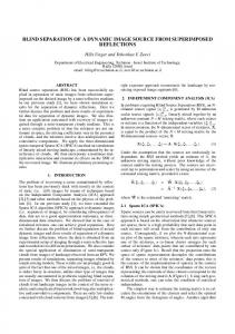
In this section, some modulation codes are designed to ensure that the transmitted signals satisfy the constraints listed in Theorem 1. In these modulation code schemes, the modulation makes part of the encoding process and it introduces redundancy by expanding the signal constellation. This means that a modulation memory is introduced in a controlled way with the purpose of keeping the orthogonality between nonlinear combinations of the transmitted signals. This constitutes a new application of modulation codes, since they are used to ensure some statistical properties associated with the channel nonlinearities. Moreover, the code redundancy could also be explored in the symbol recovery process to provide Bit Error Rate (BER) improvements, by exploiting the fact that introduced redundancy imposes some constraints on the symbol transitions. This subject will be investigated in future works. The modulated signals are characterized by Discrete Time Markov Chains (DTMC) with Rm states, given by the PSK symbols ar = {Am · e j2π (r−1)/Rm }, for r = 1, 2, ..., Rm , where Am is the amplitude of the signal of the mth user. The state transitions are defined (1) (2) (k ) by a block of km bits, denoted by Bn = {bn , bn , ..., bn m }, where (k) bn , for k=1, ..., km , is uniformly distributed over the set {0, 1} and (k) 2km < Rm . In addition, it is assumed that bn (k=1, ..., km ) are mutually independent. For each of the Rm states, the block of bits Bn defines 2km equiprobable possible transitions. Therefore, the coding imposes some restrictions on the symbol transitions. For each state,
there is Rm − 2km not assigned transitions. The code rate of the mth user is then given by (km /lm ), where lm = log2 Rm . Let us denote by T = {Tr1 ,r2 }, with r1 , r2 ∈ {1, 2, ..., Rm } the Transition Probability Matrix, Tr1 ,r2 being the probability of a transition from the state r1 to the state r2 . Note that ∑Rr2m=1 Tr1 ,r2 = 1

1512

15th European Signal Processing Conference (EUSIPCO 2007), Poznan, Poland, September 3-7, 2007, copyright by EURASIP

Current State

a1

Next State

•

bn(1)=1

a2

•

bn(1)=0

bn(1)=0

bn(1)=1

a3

bn(1)=0

•

bn(1)=1

bn(1)=0

a4

•

bn(1)=1

•

a1

•

a2

•

a3

•

a4

The results of this section may be summarized in the following corollary. Corollary 1: If the following conditions hold for all the users: (i). the transition probability matrix corresponds to an irreducible and aperiodic DTMC; (ii). ∑Rr1m=1 Tr1 ,r2 = 1, ∀ r2 , 1 ≤ r2 ≤ Rm ;

and, in addition, equations (10) are verified for (M − 1) users ∀ τ ∈ ϒ, then all the conditions of Theorem 1 are satisfied and, therefore, the covariance matrix C(τ ) is diagonal ∀ τ ∈ ϒ.

It should be highlighted that equations (10) only depend on the matrix T and the constellation order. That means that the transition probability matrices can be a priori designed to verify these equations. In the Appendix, some examples of matrices verifying these constraints are listed, with the corresponding admissible delays.

Fig. 1. Miller Code State diagram. and Tr1 ,r2 ∈ {0, 1/2km }. So, the matrix T defines which are the possible state transitions for each state. An example of mapping from the bits Bn to the corresponding PSK symbols is illustrated in Fig. 1 for a 4-PSK signal, where {a1 , a2 , a3 , a4 } are the constellation symbols (states) and km = 1. This state diagram corresponds to the run-length-limited code known as Miller Code, associated with the transition probability matrix T2,B given in (20). The Miller Code is widely used in digital magnetic recording and in Binary-PSK carrier modulation systems [8]. Similar state diagrams can be obtained for the other transition probability matrices given in the Appendix. According to Theorem 2, if all the users transmit uniformly distributed PSK signals, then conditions of Theorem 1 are verified for τ = 0. So, the following theorem proposes some constraints in the transition probability matrix T in such a way that the corresponding user transmits an uniformly distributed PSK signal. Theorem 3: Let us assume that the DTMC associated with the coding is irreducible and aperiodic. If ∑Rr1m=1 Tr1 ,r2 = 1, for 1 ≤ r2 ≤ Rm , then, for a large number of time steps, the average fraction of time steps in which the DTMC is in the state ar1 converges to 1/Rm , for 1 ≤ r1 ≤ Rm . Proof: The aperiodicity and irreducibility properties assure that [14]: (i) all the limiting probabilities of a DTMC exist and are positive, (ii) the stationary distribution exists and is unique, and (iii) the limiting probabilities distribution is equal to the stationary distribution. So, the limiting probabilities P = [p1 p2 ... pRm ] can be obtained by solving the following system of equations: 

P T = P, Rm pr = 1. ∑r=1

(8)

Now we develop some restrictions to the transition probability matrix so that the conditions of Theorem 1 be verified for τ 6= 0. Let Trn1 ,r2 be the (r1 , r2 )th entry of Tn . By definition, Trn1 ,r2 represents the probability of being in the state ar2 after n transitions, supposing that the current state is ar1 . So, we may write: h i 1 T τ E skm (n + τ )slm (n) = a T ak , Rm l

(9)

h iT where a = [a1 , a2 , ... aRm ]T and ak = ak1 , ak2 , ... akRm . Thus, the conditions (iii) and (iv) of Theorem 1 can be rewritten as: aT2 Tτ a = 0

©2007 EURASIP

and

where the matrices Ri·· , and R··k are respectively the first and thirdmode slices of R. Provided that the conditions of Corollary 1 are satisfied, these slice matrices can be expressed respectively by: Ri·· = Hdiagi [Cd ]HH

and

R··k = Cd diagk [H∗ ]HT ,

aT Tτ a = 0.

(10)

(12)

where the rows of the matrix Cd ∈ CT ×MV contain the diagonal components of C(τ ) and diagi [A] is the diagonal matrix formed from the ith row of A. So, the unfolded matrices are given by: R1 = (Cd  H) HH

and

R3 = (H∗  Cd ) HT ,

(13)

where  denotes the Khatri-Rao (column-wise Kronecker) product. The following theorem imposes a sufficient condition for the uniqueness of the considered blind estimation problem. ˆ a, H ˆ b ) and Theorem 4: Let the two pairs of matrices (H 0 ˆ0 ˆ (Ha , Hb ) be solutions to (13) for a given matrix Cd . If 2kH + kCd ≥ 2MV + 2,

It can be easily verified that if ∑Rr1m=1 Tr1 ,r2 = 1, then P = [1/Rm ... 1/Rm ] is a solution of the system (8). And finally, it can be proved (the proof is omitted due to a lack of space) that if the limiting probability of a state ar1 exists, then it is equal to the long-run time average spent in the state ar1 , i.e. for a large number of time steps, the average fraction of time steps that the DTMC spends in the state ar1 converges to the limiting probability of the state ar1 . 

aT Tτ a2 = 0,

5. CHANNEL ESTIMATION ALGORITHM Let us denote respectively by R1 ∈ CNT ×N and R3 ∈ CNT ×N the first and third-mode unfolded matrices of the tensor R, defined as:     R1·· R··1     R1 =  ...  , R3 =  ...  , (11) RT ·· R··N

(14)

ˆa=H ˆ 0a Λ and H ˆb=H ˆ 0b Λ−1 , where Λ is a MV × MV diagonal then H matrix and kA is the k-rank of matrix A, i.e. the greatest integer k such that every set of k columns of A is linearly independent. Proof: The proof of the above theorem is a direct result of the ˆ a, H ˆ b , Cˆd ) and(H ˆ 0a , H ˆ 0b , Cˆd 0 ) Kruskal Theorem [15]. Denoting by (H two solutions of (13) for Cd unknown, the Kruskal Theorem says ˆa=H ˆ 0a ΠΛa , H ˆb=H ˆ 0b ΠΛb that if kH + kH∗ + kD ≥ 2MV + 2, then H 0 and Cˆd = Cˆd ΠΛc , where Λa , Λb and Λc are diagonal matrices such that Λa Λb Λc = IMV and Π is a permutation matrix. If we assume 0 that Cd is known, then Cˆd = Cˆd = Cd and, therefore, Π = IMV , −1 Λc = IMV and Λb = Λ−1 a =Λ . The scaling ambiguity in the channel estimation introduced by the matrix Λ does not represent an effective problem, as it can be removed by a gain control at the receiver. In the Appendix, some examples of configurations of transition probability matrices for 2 users are shown, verifying kCd = MV . In this case, (14) becomes min(I, MV ) ≥ MV /2 + 1. The channel estimation is obtained by using the ALS algorithm [9, 10], the principle of which is to estimate, in the least square sense, a subset of the parameters by using a previous estimation of

1513

15th European Signal Processing Conference (EUSIPCO 2007), Poznan, Poland, September 3-7, 2007, copyright by EURASIP

0

other subsets of parameters. This process continues until the convergence of the parameters is achieved. The ALS algorithm is monotonically convergent but it may require a large number of iterations to converge [16]. For the proposed technique, each ALS iteration corresponds to two updating steps. It computes two estimates, deˆ a and H ˆ b , for the matrices H and H∗ , respectively, while noted by H the matrix Cd is assumed to be known, due to the fact that the matrices C(τ ) only depend on the modulation codes and the transmission ˆ a is power of the users. The algorithm does not take the fact that H ˆ b into account. The channel estimation the complex conjugate of H problem is solved by minimizing the following least squares cost function:

2
2
T

ˆ

ˆ ˆ ˆ T ˆ ˆ J = R 1 − C d  H a H b = R 3 − H b  C d H a , F

F



 (it−1) †

ˆa Cd  H

ˆ1 R

T

,

−4

NMSE (dB)

−6 −8 −10 −12 −14 −16 −18

(15)

−20 0

ˆ 1 and R ˆ 3 are the sample estimated unfolded matrices and where R k · kF denotes the Frobenius norm. Thus, the it th iteration of the ALS algorithm can be described by the following steps: ˆ (it) = H b

Config. 1 Config. 2 Config. 3 Config. 4

−2

5

10

15

20 SNR (dB)

25

30

(16)

2 Ns=100 Ns=300 Ns=500 Ns=1000 Ns=5000 Ns=10000

0

† T ˆ (it)  Cd R ˆ3 H b

,

−4

(17) NMSE (dB)

=



† ˆ (0) ˆ (0) where H a and Hb are I × MV Gaussian random matrices and (·) denotes the pseudo-inverse. This process continues until the convergence of the estimated parameters is achieved. Each iteration of this ALS algorithm corresponds to about (MV + 8MV2 )2IT + 2I 2 T MV + 22 3 2 3 MV + 2MV multiplications. Three channel estimates can be then (it) ˆ a , (H ˆ (it) )∗ and 0.5 · [H ˆ (it) ˆ (it) ∗ obtained: H a + (Hb ) ]. The final chanb nel estimate is chosen as the one providing the small value of the cost function (15).

6. SIMULATION RESULTS In this section, the proposed channel estimation method is evaluated by means of computational simulations. The considered channel is a memoryless MIMO Wiener filter corresponding to the model of an uplink channel of a Radio Over Fiber (ROF) multiuser communication system [4]. The wireless interface is a memoryless I × M MIMO linear channel, consisting in an uniform spaced array of I antennae. The antennae are half-wavelength spaced and the transmitted signals are narrowband with respect to the array aperture. Moreover, the propagation scenario is characterized by two users, the angles of arrival of which are 30◦ and 70◦ . The E/O conversion in each antenna is modelled by the linear-cubic polynomial [4]: −0.291x + 1.078|x|2 x. The used modulation is 4-PSK and all the results were obtained via Monte Carlo simulations using NR = 100 independent data realizations. The channel estimation method is evaluated by means of the (Normalized Mean Squared Error) NMSE of the estimated channel parameters, defined as: eH =

1 NR

NR

ˆ l k2 k H−H F 2 k H k l=1 F

∑

(18)

ˆ l ∈ CN×MV reprewhere k · kF denotes the Frobenius norm and H th sents the channel matrix estimated at the j Monte Carlo simulation. Fig. 2 shows the NMSE versus SNR for the configurations of transition probability matrices given in Table 1 of the Appendix, for M = 2, I = 4, T = 5 and Ns = 3000, Ns being the length of the data block used in the estimation of the covariance matrices. We remark that all the tested schemes provide roughly similar NMSE

©2007 EURASIP

40

Fig. 2. NMSE versus SNR using the configurations of transition probability matrices of Table 1, for M=2, I=4, T=5 and Ns = 3000.

−2

ˆ (it) H a

35

−6 −8 −10 −12 −14 −16 −18 −20 0

5

10

15

20

25

30

35

40

SNR (dB)

Fig. 3. NMSE versus SNR for various values of Ns using the Config. 2, M = 2, I = 4 and T = 5.

performances. In this case, the ALS algorithm takes approximately 15 iterations to achieve the convergence . The influence of the data block length Ns used in the estimation of the covariance matrices, is illustrated in Fig. 3. It shows the NMSE versus SNR using the Config. 2 of Table 1, with M = 2, I = 4 and T = 5. The quality of the channel estimation can be considerably improved by increasing the value of Ns , which indicates that the errors in the estimation of the covariance matrices constitute one of the main sources of the degradation in this channel estimation technique. In fact, if the theoretical values of the covariance matrices R(τ ) are used, the estimation algorithm can attain very low NMSE values, limited by the machine precision. Moreover, we have also found that the number of ALS iterations needed to achieve the convergence decreases when Ns increases. It should be highlighted from these results that the proposed channel estimator has a good robustness to AWGN, having no great performance degradation for low SNR’s. Fig. 4 shows the Symbol Error Rate (SER) versus SNR provided by the Minimum Mean Square Error (MMSE) receiver, given h i−1 ˆ MMSE = C(0) H ˆ H HC(0) ˆ ˆ H + σ 2 II by W H ∈ CMV ×N . We have

used Config. 2, M = 2, I = 4, T = 5 and Ns = 3000. In order to have a performance reference for our estimation technique, we have also simulated the MMSE receiver assuming perfect channel knowledge. Note that the SER performance using the estimated channel is very close to the one using the perfect channel.

1514

15th European Signal Processing Conference (EUSIPCO 2007), Poznan, Poland, September 3-7, 2007, copyright by EURASIP

Table 1. Examples of Configurations of transition probability matrices for 2 users. Config.

User 1

User 2

1

T1,A

T2,B

2

T1,A

T2,A

3

T1,B

T2,B

4

T1,B

T2,A

verify conditions (i) and (ii) of Corollary 1. The identifiability test in Theorem 4 depends on the covariance matrices C(τ ), for τ ∈ ϒ, which can be calculated from the transition probability matrices by using (10) and: h i 1 H τ ∗ E skm (n + τ )sl m (n) = a T ak . Rm l

(21)

Thus, it can be verified that the configurations of transition probability matrices for 2 users given in Table 1 verify kCd = MV . The corresponding admissible delays are ϒ = {0, 1, ..., T − 1}, with T ≥ 4. REFERENCES

0

10

[1] A. Ziehe, M. Kawanabe, S. Harmeling, and K.-R. Muller, “Blind separation of post-nonlinear mixtures using linearizing transformations and temporal decorrelation,” J. of Machine Learning Research, vol. 4, no. 7-8, pp. 1319–1338, 2003.

−1

10

−2

[2] S. Z. Pinter and X. N. Fernando, “Estimation of radio-over-fiber uplink in a multiuser CDMA environment using PN spreading codes,” in Canadian Conf. on Elect. and Comp. Eng., May 1-4, 2005, pp. 1–4.

SER

10

−3

10

[3] X. N. Fernando and A. B. Sesay, “Higher order adaptive filter based predistortion for nonlinear distortion compensation of radio over fiber links,” in Intern. Conf. on Comm. (ICC), New-Orleans, LA, USA, June 2000, vol. 1/3, pp. 367–371.

−4

10

−5

10

[4] X. N. Fernando and A. B. Sesay, “A Hammerstein-type equalizer for concatenated fiber-wireless uplink,” IEEE Trans. Vehicular Tech., vol. 54, no. 6, pp. 1980–1991, 2005.

Estimated Channel Perfect Channel

−6

10 −10

−5

0

5

10

15

[5] W.I. Way, “Optical fiber based microcellular systems. An overview,” IEICE Trans. Commun., vol. E76-B, no. 9, pp. 1091–1102, Sept. 1993.

SNR (dB)

Fig. 4. SER versus SNR using the Config. 2, M = 2, I = 4, T = 5 and Ns = 3000.

[6] A. J. Redfern and G. T. Zhou, “Blind zero forcing equalization of multichannel nonlinear CDMA systems,” IEEE Trans. Sig. Proc., vol. 49, no. 10, pp. 2363–2371, Oct. 2001. [7] N. Petrochilos and K. Witrisal, “Semi-blind source separation for memoryless Volterra channels in UWB and its uniqueness,” in IEEE Workshop on Sensor Array and Multichannel Proc., 12-14 Jul. 2006, pp. 566–570.

7. CONCLUSION The problem of blind estimation of memoryless multiuser Volterra channels has been studied in this paper. The proposed method is based on the PARAFAC decomposition of a tensor formed of spatiotemporal covariance matrices. Some constraints for the transmitted signals are developed to ensure the application of the PARAFAC analysis, using a two-step version of the ALS algorithm. Modulation codes are used to achieve these constraints, constituting a new application of this kind of coding. The proposed technique was applied to the identification of an uplink channel in a ROF multiuser communication system, providing good and consistent performances. The proposed blind identification method is robust to AWGN and the estimation errors of the covariance matrices are the main source of the performance degradation. In future works, other estimation algorithms will be tested and the impact of the modulation codes in the bit recovery process will be investigated. A. APPENDIX - EXAMPLES OF CONFIGURATIONS OF TRANSITION PROBABILITY MATRICES As pointed out, the transition probability matrices can be a priori designed to verify the conditions listed in Corollary 1. In the following, we present some examples of such matrices corresponding to 1/2-code rate for 4-PSK signals. It can be proved by mathematical induction that the following matrices: 

1  0 T1,A = 0.5   0 1

1 1 0 0

0 1 1 0

  0   0  , T = 0.5   1  1,B 1

0 0 1 1

  0  0   , T = 0.5   1  2,B 1

0 0 1 1

1 0 0 1

1 1 0 0

 0 1   , (19) 1  0

verify all the conditions of Corollary 1 ∀τ ∈ N. In this case a = [1 j − 1 − j]T . In addition, 

1  1 T2,A = 0.5   0 0

1 0 1 0

0 1 0 1

©2007 EURASIP

1 0 1 0

0 1 0 1

 1 1   (20) 0  0

[8] J. G. Proakis, Digital Communications, McGraw-Hill, 4rd edition, 2001. [9] R. A. Harshman, Foundations of the PARAFAC procedure: Models and conditions for an “explanatory” multimodal factor analysis, UCLA Working Papers in Phonetics, 16 edition, Dec. 1970. [10] N. D. Sidiropoulos, G. B. Giannakis, and R. Bro, “Blind PARAFAC receivers for DS-CDMA systems,” IEEE Trans. Sig. Proc., vol. 48, no. 3, pp. 810–822, March 2000. [11] I. B. Djordjevic, B. Vasic, and V. S. Rao, “Rate 2/3 modulation code for suppression of intrachannel nonlinear effects in high-speed optical transmission,” IEE Proc.-Optoelectron., vol. 153, no. 2, pp. 87–92, Apr 2006. [12] Y. Rong, S. A. Vorobyov, A. B. Gershman, and N. D. Sidiropoulos, “Blind spatial signature estimation via time-varying user power loading and parallel factor analysis,” IEEE Trans. Sig. Proc., vol. 53, no. 5, pp. 1697–1709, May 2005. [13] A. Y. Kibangou, G. Favier, and M. M. Hassani, “Blind receiver based on the PARAFAC decomposition for nonlinear communication channels,” in Proc. Colloque GRETSI, Louvain-la-neuve, Belgium, Sept. 2005, pp. 177–180. [14] O. Haggstrom, Finite Markov Chains and Algorithmic Applications, Cambridge University Press, 2002. [15] J. Kruskal, “Three way arrays: Rank and uniqueness of trilinear decomposition with applications to arithmetic complexity and statistics,” Linear Algebra Appl., vol. 18, pp. 95–138, 1977. [16] R. Bro, Multi-way analysis in the food industry: Models, algorithms and applications, Ph.D. thesis, University of Amsterdam, Amsterdam, 1998.

1515