BLIND SEPARATION OF A DYNAMIC IMAGE SOURCE FROM SUPERIMPOSED REFLECTIONS Hilit Unger and Yehoshua Y. Zeevi Department of Electrical Engineering, Technion - Israel Institute of Technology, Haifa 32000, Israel email:
[email protected],
[email protected]
ABSTRACT Blind source separation (BSS) has been successfully applied in separation of static images from reflections superimposed on the desired image by a semi-reflective medium. In our previous study [1], we have shown simulation results for the separation of dynamic reflections. Here we further discuss this problem and show results of experimental data for separation of dynamic images. We also illustrate an application concerned with recovery of images acquired through a semi-transparent cloudy medium. This is a more complex problem in that the mixtures are not stationary in space, the mixing coefficients vary in the presence of clouds, and the mixtures involve also multiplicative and convolutive components. We apply the three-dimensional spatio-temporal Sparse ICA (SPICA) method on simulations of linearly mixed moving landscape, contaminated by the interference of clouds. We then incorporate a nonlinear multiplicative interaction and examine its effects on the SNR of the recovered image. We illustrate preliminary promising results. 1. INTRODUCTION The problem of recovering a scene contaminated by reflections has been previously dealt with mostly in the context of static (i.e. still) images by means of techniques based on the Independent Component Analysis (ICA) approach [2],[3] and other methods based on the physics of the problem [4]. In our previous study [1], we have extended the Sparse ICA algorithm (SPICA) approach to dynamic images (i.e. sequences of images), by considering subsequences of data, that are to a good approximation stationary, as threedimensional data structures. We showed that in the case of simulated mixtures one can achieve good separation. Here we further discuss the problem of blind separation of mixed dynamic images and show results of separation of a dynamic image from reflections, where the data is obtained from an experimental setup of imaging through a semi-reflective lens and recorded at two different polarizations. We also consider the special application of elimination of semi-transparent clouds from images of landscape observed from an RPV. We present results of simulations, separating images obtained by simple mixing models; These results are surprisingly good in spite of the fact that one of the mixed images, i.e. the clouds, is rather fuzzy in structure, unlike other type of images that are usually encountered in problems requiring blind separation of images. We then discuss the problem of removal of clouds from landscape images in the context of the more realistic and complicated framework involving also multiplicative and convolutive components. There are only few studies concerned with cloud removal from images [5],[6]. The mul-
tiple exposure approach reconstructs the landscape by mosaicing exposed image segments [6]. 2. INDEPENDENT COMPONENT ANALYSIS (ICA) In problems requiring Blind Source Separation (BSS), an Nchannel sensor signal {xi }Ni=1 is generated by M unknown scalar source signals {si }M i=1 , linearly mixed together by an unknown constant N × M mixing matrix, where each source or mixture is a function of the independent variables {ξi }ki=1 . In matrix notation, the N-dimensional vector of mixtures, X , is equal to the product of the N × M mixing matrix by the M-dimensional sources vector, S : X (ξ1 , ξ2 , . . . , ξk ) = A
· S (ξ1 , ξ2 , . . . , ξk ).
(1)
Under the assumption that the sources are statistically in˜ the dependent, the BSS method yields an estimate of A, unknown mixing matrix, without prior knowledge of the sources and/or the mixing process. The sources are recovered (up to permutation and scale) by using an inverse of the estimated mixing matrix, provided it exists: S ˜ (ξ1 , ξ2 , . . . , ξk ) = W ˜ = A˜ where W ˜
· X (ξ1 , ξ2 , . . . , ξk ) −1
· X (ξ1 , ξ2 , . . . , ξk ),
(2)
is the estimated ’unmixing’ matrix.
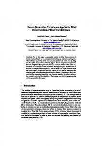
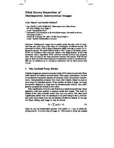
2.1 Sparse ICA (SPICA) Sparse sources can be easily recovered from their linear mixtures using simple geometrical methods [7],[8]. This SPICA approach is based on the observation that whenever sources are sparse, there is a high probability that each data point in each mixture will result from the contribution of only one source. Consequently, if we plot the N-dimensional scatter plot of the sparse mixtures, wherein each axis represents one of the mixtures, a co-linear cluster emerges for each subset of mixtures’ data points that are contributed by one source only (Figure 1c). Recall that the projection onto the space of sparse representation decouples the contributions of the sources to most of the mixtures’ data points; this is the essence of the implementation of sparsity in the context of BSS. It can be shown that the coordinates of the vectors representing the centroids of these clusters correspond to the columns of the mixing matrix A (Figure 1). Using such geometrical methods, one can relax the condition of statistical independence. The simplest way to estimate the mixing matrix is to calculate the orientations of the clusters and select the optimal M angles from the histogram of angles. Another algorithm
projects the data points onto a hemisphere, then uses clustering (such as Fuzzy C-means) in order to recover the orientations [8]. Other methods, such as the well-known Infomax [9] use a maximum-likelihood-based approach [10]. After the orientations have been calculated, the sources can be estimated by using eq. (2). 2.5
2.5
2
2
1.5
1
1.5
1.5
1 1 0.5
0.5 mixture 2
0.5 0 0
0
−0.5 −0.5 −1
−0.5
−1
−1.5
−1
−1.5
−2
−2.5
0
20
40
60
80
100
120
140
160
180
200
−2
−1.5
0
(a) Sources
20
40
60
80
100
120
140
160
(b) Mixtures
180
200
−1
−0.5
0 0.5 mixture 1
1
1.5
2
(c) Scatterplot
Figure 1: An example of three sparse sources (a) mixed into two mixtures (b). The orientations of three lines in the scatter plot correspond to the columns of the mixing matrix.
more degrees of freedom that can be exploited in their design. However, nonseparable wavelets are much more complex to deal with [11] and their application in the context of sparsification is therefore beyond the scope of this study. 2.2.3 Source Separation using the WPT After the mixture signals are decomposed into WP-tree using the WPT [8], we search for the most sparse node. A quality criterion that assigns high values for sparse nodes and lower values for less sparse nodes is computed for every node [8]. Common choices for such quality criteria are entropy or global distortion. The best node (or the top few nodes) is chosen and used as input data for the geometrical BSS algorithm. Using the WPT has another advantage: because of downsampling in the process of the transform, the number of data points in each node is significantly smaller than the number of mixture signals data points. This reduction in the number of data points speeds up the processing. 1
2
0.9
1.5
0.8
2.2 Sparse Decompositions
1
0.7 0.5 0.6 0 0.5
2.2.1 Overcomplete Representations
−0.5 0.4 −1 0.3
Natural images and image sequences are not typically sparse. In order to exploit the geometrical method of SPICA, we have to first apply a sparsification transformation, and then apply the geometrical algorithm on the transformed signals. It has been shown that for a wide range of natural images, smoothed derivative operators yield a good sparsification results [3]. However, an overcomplete representation obtained, for example, by the Wavelet Packet transform (WPT) matches better the specific structure of a given set of images and thereby yields better sparsification [8]. The latter facilitates and improves the estimation of the mixing matrix. The local nature of the wavelet-type transforms can highlight specific features of distributions (such as the distinct orientations in a scatter plot) based on a subset of data points of the transformed signal. Such highly structural distributions are not clearly present in the highly correlated non-transformed signal. 2.2.2 WP transform The Wavelet Packet family consists of the triple-indexed family of functions:
ϕ jnl (ξi ) = 2 j/2 ϕn (2 j ξi − l) , j, l ∈ Z, n ∈ N ξ1 ≡ x, ξ2 ≡ y, ξ3 ≡ t ϕ jnl = ∏ ϕ jnl (ξi )
−1.5
0.2
−2
0.1
0
0
0.1
0.2
0.3
0.4
0.5
0.6
0.7
0.8
−2.5 −1
−0.8
−0.6
−0.4
−0.2
0
0.2
0.4
0.6
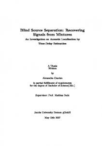
0.8
Figure 2: Left: a scatter plot of mixtures of two non-sparse images. Right: the scatter plot of a wavelet packet tree node. The arrows show the estimated centroid orientations. 3. BSS OF DYNAMIC REFLECTIONS We first apply our method in a relatively simple physical example of separation of dynamic reflections, such as video recorded through the windshield of a car or the canopy on an airborne platform. In this example the assumptions of linearity and stationarity are valid. Here, a virtual (reflected) image is superimposed on a dynamic visual scene. To this end we extend the study concerned with separation of reflections from static images [2],[3] to the case of 3D dynamic images. In the context of separation of reflections, the BSS problem usually reduces to the case of M=2 sources. The observed mixture is then given by x(ξ 1, ξ 2,t) = a11 s1 (ξ 1, ξ 2,t) + a12 s2 (ξ 1, ξ 2,t),
(3)
i
According to the formalism of the WPT, a signal is recursively decomposed into its approximation (L) and detail (H) subspaces. In the case of 2D signals, using separable wavelets, the signal is decomposed into its approximation and vertical, horizontal and diagonal details sub-images. For 3-dimensional data cube, the signal is decomposed into 8 sub-volumes. We chose to use a separable transformation, for the sake of simplicity, by transforming rows first, then columns and then time (depth) axis. Nonseparable wavelets offer important advantages in that they are inherently endowed with
(4)
where x, s1 and s2 are dynamic images, usually acquired as video sequences. It is assumed here that the dynamics of the image and of the superimposed reflections are limited to planar translation of rigid bodies. The more difficult problem of non-planar motion and rotation, as well as of non-rigid distortion are beyond the scope of this paper, and will be dealt with elsewhere. Likewise, the coefficients a11 and a12 are assumed to be constant, approximating spatial invariance and linear mixing [3]. Since the reflected light is polarized, by using a linear polarizer, the relative weights of the two mixed video sequences can be varied to yield N different mixtures of the form: xn (ξ 1, ξ 2,t) = an1 s1 (ξ 1, ξ 2,t) + an2 s2 (ξ 1, ξ 2,t) : n = 1, . . . , N .
(5)
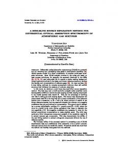
Thus, we can use two or more video sequences obtained with different polarizations and separate objects and reflections. Figure 3 shows frames from video sequences of a real data experiment in which a dynamic reflection was superimposed on a static image. As can be seen, the reflection and image are successfully separated.
clouds have a different velocity (in time) relative to the landscape. Reconstruction quality was measured by SNR (dB). The respective results are 4.5dB for the cloud sequence and 16.5dB for the landscape sequence. Although these figures of SNR do not indicate outstanding results, the visual appearance of the images is very convincing, considering the relatively complex structure of the clouds and consequently the mixtures.
Figure 3: Results of an experiment of blind separation of a static image from a superimposed dynamic reflection: frames from one mixture (top), frames from the recovered image (middle) and superimposed reflection (bottom). 4. SEPARATION OF LANDSCAPE FROM CLOUDS Images acquired using airborne cameras outfitted on an RPV are usually contaminated by the interference of clouds. In this application, it is desirable to extract a clear landscape view and separate it from the thin semi-transparent layers of clouds. This problem has hardly been dealt with in the past [5],[6]. The problem of separation of clouds from landscape is a more complex problem than the relatively simple one of separation of reflections, addressed and illustrated in section 3. To begin with, the mixtures are not spatially stationary since the mixing coefficients vary in the presence of clouds. Further, combined images recorded above the clouds do not necessarily reflect simple, strictly linear, mixing. They are rather obtained by a more complex process involving multiplicative and convolutive elements, which may affect the quality of separation. Such a complex process of mixing may be qualitatively described by: X
= AS
+ α F (S , S ∗ K ),
(6)
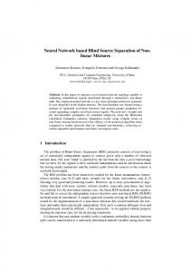
where K is a vector of the convolution kernels and F is a non-linear function of the sources and the convolved sources. In our studies with reflections and other applications of BSS, we noticed that our technique of using wavelet-type localized sparsification transformations such as the WPT renders the data to become robust with respect to weak nonlinearities and nonstationarity. The latter is due to the localized structure of the data sparsified by such transformations. We are at the present time in the process of constructing a special imaging system for the application of separation of clouds. However, as long as we do not have real data, it is reasonable to assume that α is small and apply our approach on linear mixtures of landscape and cloud images. The three images depicted in the top row of Figure 4 are taken from a sequence of linearly mixed sequences of a landscape and clouds. The
Figure 4: Top: three images from a synthetic mixture movie of landscape with clouds. Middle: three images from the movie of one extracted source. Bottom: three images from the movie of the second extracted source.
Figure 5: Left: a simulated source of clouds image. Right: the multiplicative mask created from the clouds image. To better approximate the nonlinear, multiplicative, effect that comes along with the presence of clouds in the cloudy areas, we add a mask which accounts for imaging through a cloudy medium (Figure 5). The mixing is now performed in the following way: MIX1 = a11 · MASK · landscape + a12 · clouds MIX2 = a21 · MASK · landscape + a22 · clouds.
(7)
The quality of the blind separation is now considerable compromised due to the incorporation of a multiplicative process, and the recovered images are in this case characterized by SNR of 1.4dB for the clouds and 14.1dB for the landscape sequence. Further refinement of the model awaits the analysis of real data of sequences of landscape images acquired through a thin semitransparent layer of clouds.
Figure 6: Top: three frames from a video of the recovered landscape. Bottom: three frames from the video of the recovered video of clouds. 5. DISCUSSION BSS algorithms have been shown to provide powerful means for blind separation of images in various scenarios where the mixing is approximately stationary (fixed in space) and linear. In particular it has been successful in separating images from superimposed reflections [1],[2],[3], and in separation of tissues in MRI [12]. However, problems such as recovery of a landscape imaged through a layer of semi-transparent medium have not been previously addressed in this context and have hardly been discussed in the context of other image processing approaches and algorithms [5],[6]. We show here that the physics of imaging with two polarizations, successfully implemented in separation of an image from superimposed dynamic reflections, can be instrumental in the more complex case of recovery of an image contaminated by the effects of a layer of cloud present along the pathway of the imaging device. The problem of separation of landscape images from clouds calls for models that are more complex than simple linear mixing. The combination of blind separation and blind deconvolution has recently attracted a great deal of interest in the community of ICA. It is expected that new emerging results will penetrate the field of image processing and find new applications. In this study we are in the process of further generalizing the approach, by incorporating also hard nonlinearities in the form of a multiplicative effect. This has yet to be further studied before we have a better understanding of the advantages and limitations of a generalized BSS approach. However, preliminary results such as those illustrated in the present study appear to be promising enough to encourage further investigation. Although the SNR results indicate that the separation quality is not yet good enough in the case of the non-linear model that incorporates a multiplicative mask, it seems that the localized mapping into a space of sparse representation should better deal with the spatial varying effects introduced by the map. Since our mapping may be overcomplete and its only purpose is to estimate the mixing matrix, one may consider using a combination of two dictionaries; One that incorporates the specific structure of the landscape, which in the example used by us may be based on scale-space of corner detectors. A second dictionary may account for the fractal nature of cloud structure. In spite of the less-than-optimal sparsification used in this preliminary study, the improvement achieved in
the resultant sequence of landscape allows better further processing of the data by conventional techniques of image processing, which we have not attempted to use here. We intend to test the model proposed here for the interference of the a layer of clouds on real data, using a special imaging system currently developed by us. In addition to further refinement of the model and of the sparsifying techniques, we intend to take advantage also of the fact that in the scenario under consideration there are areas that are not covered by clouds. This brings us the idea of performing the analysis block-wise, using sub-blocks of data (as proposed in [3]). Mosaicing of segments reduced from multiple exposures [6] can also be incorporated and further improve our results. Acknowledgement: Research supported in part by the HASSIP Research Network Program HPRN-CT-2002-00285, sponsored by the European Commission, by the Ollendorff Minerva Center, and by the Fund for promotion of research at the Technion. REFERENCES [1] H. Unger and Y. Y. Zeevi. Blind separation of spatiotemporal data sources. In ICA04, pages 962–969, 2004. [2] H. Farid and E. H. Adelson. Separating reflections and lighting using independent components analysis. In CVPR, pages 1262–1267, 1999. [3] A.M. Bronstein, M.M. Bronstein, M. Zibulevsky, and Y.Y. Zeevi. Blind separation of reflections using sparse ICA. In ICA03, pages 227–232, Nara, Japan, apr 2003. [4] Y.Y. Schechner, J. Shamir, and N. Kiryati. Blind recovery of transparent and semireflected scenes. In CVPR, pages 1038–1043, 2000. [5] H. Snoussi and A. Mohammad-Djafari. Fast joint separation and segmentation of mixed images. Journal of Electronic Imaging, 13(2):349–361, 2004. [6] S.C. Liew, M. Li, L.K. Kwoh, P.C., and H. Lim. ”Cloud-free” multi-scene mosaics of spot images. In IGARSS98, pages 1083–1085, Seattle, WA, USA, Jul 1998. [7] M. Zibulevsky and B.A. Pearlmutter. Blind source separation by sparse decomposition in a signal dictionary. Neural Computation, 13(4):863–882, 2001. [8] P. Kisilev, M. Zibulevsky, and Y.Y. Zeevi. A multiscale framework for blind separation of linearly mixed signals. J. Mach. Learn. Res., 4:1339–1363, 2003. [9] A.J. Bell and T.J. Sejnowski. An informationmaximization approach to blind separation and blind deconvolution. Neural Computation, 7(6):1129–1159, 1995. [10] J.F. Cardoso. Infomax and maximum likelihood for blind source separation. IEEE Signal Processing Letters, 4(4):112–114, April 1997. [11] D. Stanhill and Y.Y. Zeevi. Two-dimensional orthogonal wavelets with vanishing moments. IEEE Transactions on Signal Processing, 44(9):2579–2590, 1996. [12] A.M. Bronstein, M.M. Bronstein, M. Zibulevsky, and Y.Y. Zeevi. ”Unmixing” Tissues: Sparse Component Analysis in Multi-Contrast MRI. submitted to ICIP 2005.