Boost Phase Tracking with an Unscented Filter - CiteSeerX

Boost phase tracking with an unscented filter James R. Van Zandt a MITRE

a

Corporation, MS-M210, 202 Burlington Road, Bedford MA 01730, USA

ABSTRACT

Boost phase missile tracking is formulated as a nonlinear parameter estimation problem, initialized with an unscented transformation, and updated with a scaled unscented Kalman filter. Keywords: unscented transform, extended Kalman Filter, scaled unscented filter, tracking, boost phase

1. INTRODUCTION The subject of this paper is the estimation of launch parameters (principally latitude, longitude, azimuth, and launch time) of a missile during boost phase. Several methods have been proposed for tracking boosting missiles, including constant gain alpha-beta-gamma or constant acceleration filters,1 filters with dynamic booster models,2–4 or by fitting to a known profile (e.g. tabulated values of altitude and downrange distance as a function of time). 5,6 The latter can diverge if the missile does not follow the expected trajectory, as in using a different loft or if no appropriate profile is available for the missile in question. It is also a batch process, so it must be repeated as new observations become available. The other methods do not directly yield the launch parameters. This paper explores an intermediate method, where a realistic dynamic model is used for the booster (in particular, one with a natural description of lofted or depressed trajectories ), but the state parameters to be estimated are the initial conditions for the launch. Our goal is to find a maximum likelihood estimate of the trajectory parameters. In this work, an Unscented Transformation7,8 is used to initialize this estimate from the first observation. As subsequent observations become available, a filter is used to recursively update the parameter estimate. For linear systems, the Kalman Filter 9 (KF) maintains a consistent estimate of the first two moments of the state distribution: the mean and the variance. Since our observation function (that is, the function that predicts the target state at the observation time based on the current estimate of the trajectory parameters) is nonlinear, we need a nonlinear tracking filter. The Extended Kalman Filter (EKF)10 allows the Kalman filter machinery to be applied to nonlinear systems. In the EKF, the state distribution is approximated by a Gaussian random variable, and is propagated analytically through the first-order linearization (a Taylor series expansion truncated at the first order) of the nonlinear function. This linearization can introduce substantial errors in the estimates of the mean and covariance of the transformed distribution, which can lead to sub-optimal performance and even divergence of the filter. In this work, the more accurate scaled Unscented Kalman Filter11 (UKF) is used to update the model parameter estimates. Section 2 describes the Unscented Kalman Filter. Section 3 discusses the missile flyout model and filter initializa­ tion. Section 4 mentions some implementation considerations. Section 5 illustrates the performance of the method. Section 6 summarizes the results. Appendix A provides the derivation of the flyout model. c �2002 The MITRE Corporation. ALL RIGHTS RESERVED

2. THE SCALED UNSCENTED KALMAN FILTER Julier and Uhlmann have described the unscented transformation (UT) which approximates a probability distribution using a small number of carefully chosen test points.7,8 These test points are propagated through the true nonlinear system, and allow estimation of the posterior mean and covariance accurate to the third order for any nonlinearity. ˆ and covariance As originally described, the UT approximates an n dimensional random variable x with mean x P by 2n + 1 samples X0 . . . X2n with weights W0 . . . W2n as follows: X0

=

W0

=

Xi

=

Xi+n

=

Wi

=

ˆ x

(1)

κ n+κ �� � ˆ+ x (n + κ)P �� �i ˆ− x (n + κ)P

(2)

i

Wi+n =

1 2(n + κ)

i = 1···n

(3)

i = 1···n

(4)

i = 1 · · · n,

where κ is any number, positive or negative, provided n + κ �= 0, and �� � (n + κ)P

(5)

(6)

i

is the ith row of the matrix square root A of P, such that P = AT A. Each sample point is first transformed as Yi = f (Xi ).

(7)

The mean of the transformed distribution is then estimated as ˆ= y

2n � i=0

and its covariance as Pyy =

2n � i=0

Wi Y i ,

(8)

ˆ ˆ T. Wi {Yi − y}{Y i − y}

(9)

With this method, as the dimension of the state space increases, the radius of the sphere that bounds all the sample points also increases. The mean and covariance of the points still match those of the a priori distribution, but they may seriously oversample the tails of the distribution. To control this, we use Julier’s method of scaling the sample points.11 The new sample points and the weights used for finding the mean are Xi� Wi�

=

X0 + α(Xi − X0 ) � W0 /α2 + 1 − 1/α2 = Wi /α2

(10) i=0 i �= 0

The covariance is found using a modified set of weights � W0 /α2 + 2 − 1/α2 − α2 + β Wi�� = Wi /α2

i=0 , i �= 0

(11)

(12)

where β is another adjustable parameter. The mean and covariance are estimated as Yi�

=

f (Xi� )

(13)

ˆ� y

=

2n �

Wi� Yi�

(14)

2n �

ˆ � }{Yi� − y ˆ � }T . Wi�� {Yi� − y

(15)

i=0

P�yy

=

i=0

It remains to set the adjustable parameters κ, α, and β. We follow Julier’s recommendation of β=2

(16)

to capture part of the fourth order term in the Taylor series expansion of the covariance. We choose √ α = 1/ n

(17)

to make the sample diameter independent of the state size. The UT effectively estimates the transformed mean and variance by statistical regression,12 so we expect the estimate to be more accurate if the prior distribution is approximately uniformly sampled. The estimated covariance P�yy is guaranteed to be positive semidefinite if all the untransformed weights are non-negative, which establishes the condition κ > 0. We also want the transformed weights to be non-negative for robustness (if one sample point has a substantially negative weight, then a nonlinearity can lead to a biased estimated mean and an inflated covariance), which establishes the stricter condition κ > n 2 − n. We actually choose to make all the transformed weights equal, so that κ = n2 − n/2.

(18)

For n = 16, we have α = 1/4, κ = 248, and W0� = Wi� = 1/33. The Unscented Kalman Filter13,14 (UKF) uses the UT for both the transformations (process model and obser­ vation function) required by a Kalman filter. It provides a Minimum-Mean-Squared Error (MMSE) estimate of the state of a nonlinear discrete time system x(k + 1) = f [x(k), u(k), v(k), k] z(k) = h[x(k), u(k), k] + w(k),

(19) (20)

where x(k) is the state of the system at time k, f [k] and h[k] are the possibly nonlinear system and observation functions, u(k) is the input vector, v(k) is the process noise, z(k) is the observation, and w(k) is additive measurement noise. v and w are assumed zero mean and � � E v(k)vT (j) = δkj Q(k), (21) � � T E w(k)w (j) = δkj R(k), (22) � � T E v(k)w (j) = 0, ∀k, j. (23) An augmented covariance matrix is constructed with P, Q, and R on the diagonal. Eqs. 10-12 then provide sample points Xi� (k + 1|k) that specify not only x but also v and w. ˆ (k + 1|k) and its covariance P(k + 1|k) are estimated as The predicted state x Xi (k + 1|k) = f [Xi (k|k), u(k), k] ˆ (k + 1|k) = x

2n � i=0

P(k + 1|k) =

2n � i=0

(24)

Wi� Xi (k + 1|k)

(25) T

ˆ + 1|k)} {Xi (k + 1|k) − x(k ˆ + 1|k)} . Wi�� {Xi (k + 1|k) − x(k

(26)

ˆ, its covariance Pzz , and the cross correlation Pxz are estimated as The predicted observation z Z(k + 1|k) = h [Xi� (k + 1|k), u(k), k + 1] ˆ(k + 1|k) = z

2n � i=0

Pzz (k + 1|k) =

2n � i=0

(27)

Wi� Zi (k + 1|k)

ˆ + 1|k)} {Zi (k + 1|k) − z(k ˆ + 1|k)} Wi�� {Zi (k + 1|k) − z(k

(28) T

(29)

Pxz (k + 1|k) =

2n � i=0

T

ˆ + 1|k)} {Zi (k + 1|k) − z(k ˆ + 1|k)} . Wi�� {Xi (k + 1|k) − x(k

(30)

ˆ The state estimate x(k|j) at time step k, and its covariance P(k|j), given all observations up to and including time step j, are updated as follows: Pνν (k + 1|k) = R(k + 1) + Pzz (k + 1|k) W(k + 1) = Pxz (k +

1|k)P−1 νν (k

(31)

+ 1|k)

(32)

ˆ + 1|k + 1) = x(k ˆ + 1|k) + W(k + 1)(z(k + 1) − z(k ˆ + 1|k)) x(k

(33)

P(k + 1|k + 1) = P(k + 1|k) − W(k + 1)Pνν (k + 1|k)W (k + 1),

(34)

T

where W is the Kalman gain. For linear functions, the UKF is equivalent to the KF. The computational complexity of the UKF is the same as the EKF, but it is more accurate and does not require the derivation of any Jacobians.

3. MISSILE FLYOUT MODEL We assume the missile has constant thrust and follows a gravity turn with zero angle of attack. That is, we assume the thrust vector is always parallel to the earth-relative velocity vector. We assume a spherical, non-rotating earth, and neglect aerodynamic drag and lift. Let r be the missile position, v be its velocity, and a t be the acceleration due to rocket thrust. The missile state obeys the differential equations given by Hough 15 (see Appendix A). dr dt dv dt dat dt

=

v

(35)

=

at + g � at U at + ω × a t 0

(36)

=

t < tf t > tf

(37)

where

µe r r3 . is the gravitational acceleration, µe = 3.986004418 × 1014 m3 /sec2 is the gravitational parameter, g=−

ω = (v × g)/v 2

(38)

(39)

is the angular rate of v and at , and tf is the burnout time. For our model, the trajectory of a single stage missile is determined by eight parameters: tlaunch = L = λ = β = U = θi = ai = af =

launch time

launch latitude

launch longitude

launch azimuth

exhaust velocity

initial tilt angle (i.e. angle from vertical)

initial acceleration magnitude

acceleration magnitude at burnout.

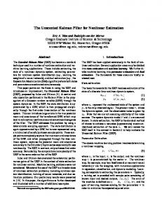
The last four parameters are characteristic of the missile. The least familiar of these is the tilt angle. Only a small range separates a tilt angle that yields an almost vertical trajectory from one that allows the missile to fall over immediately after launch, especially for a missile with low initial acceleration. The feasible values of θ i and ai are also highly correlated, as shown in Fig. 1. (Recall that for a short range missile, a zenith angle at burnout near 45 degrees gives maximum range.) The nonlinearities may be mitigated by transforming both parameters. Instead

vboost1

32 30

burnout FPA = 75 deg

28 60

26

a_i (m/sec^2)

45 24

30

22 20

initial velocity = 1 m/sec exhaust velocity = 2700 m/sec mass fraction = .91 gravity turn nonrotating spherical earth

18 16

1 mrad |

14

10 mrad |

12 0

0.002

0.004

0.006

0.008

0.01

0.012

0.014

0.016

0.018

0.02

initial tilt (radians)

Figure 1. Correlation of Initial Tilt and Acceleration Magnitude of θi we will use τi = ln(θi ), and instead of ai we will use � � ai αi = ln −1 , ge

(40)

where ge = 9.8 m/sec2 is the approximate acceleration of gravity at the earth’s surface. This helps greatly, as shown in Fig. 2. Initial values suitable for some hypothetical missiles are also shown. For those distributions, the correlation vboost

2

1.5

initial velocity = 1 m/sec exhaust velocity = 2250 m/sec mass fraction = .91 gravity turn nonrotating spherical earth

ln(a_i/(1 g) - 1)

1

0.5

0

-0.5

75 deg burnout FPA 60 45 30

notional missile parameter estimates

-1

-1.5 -18

100 urad |

-16

-14

-12

-10 ln(initial tilt)

1 mrad |

-8

10 mrad |

-6

-4

-2

Figure 2. Correlation of Transformed Initial Tilt and Acceleration Magnitude coefficient between αi and τi ranges from 0.96 to 0.99. For two stage missiles, we add two states for the initial and final acceleration magnitude of the second stage. (U is assumed to be the same for the two stages.) The first four parameters (tlaunch , L, λ, and β) are different for each launch, and can be found from the initial estimated target position r and velocity v. (Hough describes initialization using angles-only measurements. 15 )

The launch latitude and longitude are estimated together. The surface location r u = [xu yu zu ]T directly under the target is re ru = r. (41) r This is converted to a latitude and longitude with � (42) Lu = tan−1 (zu / x2u + yu2 ), λu

= tan−1 (yu /xu ).

(43)

The approximate straight-line extrapolation of the current state back to the ground (i.e. in the −v direction from r) is vrh rs = r − , (44) v·r which is similarly converted to latitude Ls and longitude λs . The launch point is then estimated as a linear interpo­ lation between these two surface points: λ = aλu + (1 − a)λs L = aLu + (1 − a)Ls ,

(45) (46)

where a ≈ .25.

The launch azimuth is estimated from the horizontal component of the target velocity vh = (r × v) × r/r 2 .

(47)

ˆ be a unit vector in the z direction. Then e ˆ=z ˆ × r/|ˆ Let z z × r| is a unit vector eastward from the current estimated ˆ = r × e/|r ˆ × e| ˆ is a unit vector northward. The launch azimuth is then position, and n � � ˆ vh · e β = tan−1 . (48) ˆ vh · n We may estimate the flight time t (hence tlaunch ) from the altitude using some further simplifications of the dynamics model, specifically vertical launch and constant gravity. The thrust acceleration magnitude a t obeys the equation a2 a˙ t = t . (49) U We can integrate to find the acceleration as a function of flight time at =

ai . 1 − ai t/U

If the acceleration at burnout is af , then the time of burnout is � � 1 1 tf = U − . af ai

(50)

(51)

Assuming a vertical trajectory and constant gravitation force of ge , we substitute this into Eq. 36 and integrate again to find the velocity v(t) = vi − ge t − U ln (1 − ai t/U ) , (52) and similarly from Eq. 35 the altitude 1 U2 h(t) = r − re = (vi + U )t − ge t2 + (1 − ai t/U ) ln (1 − ai t/U ) , 2 ai

(53)

where re is the earth radius. Eqn. 53 can be solved for t iteratively. Bringing the third t to the left hand side gives us the iteration U h − (vi + U )tk + ge t2k /2 tk+1 = − , (54) U ln(1 − ai tk /U ) ai

which converges from a wide range of starting values. With the starting value t0 =

� 2 U � 1 − e−5ai h/U , ai

(55)

two iterations suffice (e.g. giving the flight time to within one second for any altitude from 10 km to burnout). Eqns. 41-54 represent a nonlinear transformation from the estimated target state to the values of the first four parameters. However, the position and velocity of the target are not known precisely. In a practical system the target state has an uncertainty described by a covariance matrix. We really need to transform the uncertainty distribution, not just a single value. In this work, the scaled Unscented Transformation described in Section 2 is used to estimate the initial state and covariance.

4. IMPLEMENTATION In our method, each missile with a given number of stages is represented by an uncertainty region in the parameter space. To track an unknown missile, one can either initialize a single filter with a large uncertainty region to cover the region of interest or use several filters, each initialized appropriately for a different missile. Separate filters are needed in any case to accommodate both single and two stage missiles, so we have chosen the latter method. The prediction program must handle infeasible conditions, such as ai > af or ai < 0. We have chosen in both cases to integrate over a zero interval. The equation for the angular velocity of at is indeterminate when v = 0, so it is necessary to initialize the motion with a small velocity. In addition, the equation for thrust acceleration magnitude has a singularity at time t = ti + U/ai . This is why the burnout time was not chosen as a state variable—its uncertainty distribution might extend past the singularity.

5. EXAMPLE The estimation procedure was tested using a small simulation in which a missile is launched directly eastward. Its position and velocity are observed four times at four second intervals, with spherically symmetric uncertainty (one sigma) of 100 m and 100 m/sec. Initialization of latitude and longitude is shown in figure 5. The actual launch point is indicated with an asterisk. The point [Lu , λu ] directly under the target and the straight line extrapolation to the surface [L s , λs ] are shown with right- and left-pointing triangles respectively (both calculated from the the first observation mean). The state is augmented with a, the weight on the sub-target point. The augmented covariance is   1002   1002   2   100   .  1002 (56)   2   100     1002 0.12 The calculated launch points corresponding to the various sample points are shown with plus signs. The one-sigma contour of the resulting launch point estimate is shown as an ellipse. The prediction of the next observation is shown in Fig. 4. As before, the actual launch site is represented by an asterisk, the transformed sample points are shown with plus signs and the one-sigma contour of the resulting estimate is shown with the ellipse. (Several of the transformed sample points are below ground because the initial distribution of tilt and acceleration magnitude was broad enough that for some values the missile would fall over immediately after launch. This leads to a large uncertainty in the predicted slant range.) In addition, there are lines from the center of the ellipse to the mean estimated launch point and to the actual observation (whose uncertainty is too small to show up here). The updated launch point estimate is shown in Fig. 5. The prediction for the third observation is shown in Fig. 6, and the prediction for the fourth observation is added in Fig. 7. Its elevation from the launch point is intermediate between the first two predictions. The uncertainty in

LPE, type 1: Generic1Stage CU 1 track 1

30.08

30.06

30.04

latitude

30.02

30

29.98

29.96

29.94

29.92

29.9 −140.05

−140

−139.95 longitude

−139.9

−139.85

Figure 3. Initialization 4

prediction, type 1: Generic1Stage CU 1 track 1

x 10 6

5

4

altitude (m)

3

2

1

0

−1

−2 −4

−3

−2

−1

0 1 distance E (m)

2

3

4

5

6 4

x 10

Figure 4. Prediction of first measurement. predicted slant range has not improved much. The estimated launch point after three updates is shown in Fig. 8. The estimate has a bias in crossrange. ˆ T − [Lλ]T be the error in the estimated launch position, and Pll be the corresponding part of the ˆ λ] Let dll = [L estimated covariance. If the filter’s estimated covariance were accurate, then the normalized distance D2 = dT Pll−1 d

(57)

would be chi-square distributed with two degrees of freedom. The actual distribution of D for 250 Monte Carlo trials is shown in Fig. 9. Evidently, the filter underestimates the uncertainty of the launch position. The distribution of north and east components of the LPE error are shown in Fig. 10. The median errors are 252 m in latitude and 884 m in longitude. The latter is likely due to the Coriolis accelerations which were neglected above. There is an outlier with a longitude error of 7247 m. However the means of the estimated position variances are only 593 m in latitude and 1474 m in longitude, so even disregarding the outlier and the bias, the estimated variance is optimistic.

6. CONCLUSION The launch parameters for a missile have been estimated using an analytic approximation of the trajectory and an unscented Kalman filter. Transformations of the parameters were identified which substantially reduce the

LPE, type 1: Generic1Stage CU 1 track 1

30.08

30.06

30.04

latitude

30.02

30

29.98

29.96

29.94

29.92

29.9 −140.05

−140

−139.95 longitude

−139.9

−139.85

Figure 5. Estimated launch point after first update. 4

prediction, type 1: Generic1Stage CU 1 track 1

x 10 6

5

4

altitude (m)

3

2

1

0

−1

−2 −4

−3

−2

−1

0 1 distance E (m)

2

3

4

5

6 4

x 10

Figure 6. Prediction of second measurement. nonlinearities in the effective observation function. Nevertheless, the filter does not accurately update the parameter estimate. We suspect that the cross-covariance matrix is being evaluated too far from the optimal solution, so the filter overcorrects. We plan to investigate whether an iterated UKF such as that of Bellaire et al. 16,17 would improve the result. Alternatively, the problem could of course be formulated as a least-squares estimation problem and solved in a batch process with the method of Levenberg and Marquardt.18

APPENDIX A. DERIVATION OF ROCKET MODEL During boost, the thrust acceleration is almost parallel to the longitudinal axis e of the vehicle: at = a t e

(58)

dat = a˙ t + ω × at , dt

(59)

Differentiation yields the vector-differential equation

where e rotates at angular velocity ω with respect to inertial space. With constant mass flow rate and exhaust velocity U , the rate of change of thrust acceleration may be approximated by a˙ t =

a2t . U

(60)

4

prediction, type 1: Generic1Stage CU 1 track 1

x 10 6

5

4

altitude (m)

3

2

1

0

−1

−2 −4

−3

−2

−1

0 1 distance E (m)

2

3

4

5

6 4

x 10

Figure 7. Prediction of third measurement. LPE, type 1: Generic1Stage CU 1 track 1

30.08

30.06

30.04

latitude

30.02

30

29.98

29.96

29.94

29.92

29.9 −140.05

−140

−139.95 longitude

−139.9

−139.85

Figure 8. Estimated launch point after three updates. During flight in the atmosphere, a thrusting missile is generally controlled to maintain small angles of attack between the longitudinal axis e and the earth-relative velocity u = v − ω e × r, (61) . where ω e = 7.292115856 × 10−5 rad/sec is the earth rotation rate. Differentiating with respect to time, the equations of motion take the form du dv dr = − ωe × = at + aa + g(r) − ω e × v. (62) dt dt dt where aa is the aerodynamic acceleration which we will eventually neglect. Expressing the time derivative with respect to inertial space in terms of the body frame, �u� u˙ + ω × u = at + aa + g(r) − ω e × v. (63) u We remove the component parallel to u using a vector cross product: (ω × u) × u = (ω · u)u − u2 ω = (at + aa + g(r) − ω e × v) × u,

(64)

where ω · u = 0 because we assume the vehicle is stabilized in roll, so we find ω = u × (at + g − ω e × v)/u2 .

(65)

normdist

1 0.9 0.8 initialization intentionally conservative

cumulative fraction

0.7 0.6 0.5 0.4 uncertainty estimates grow more optimistic

0.3 0.2 initial 1-exp(-x**2/2) 1st update 2nd update 3rd update

0.1

1

2

3

4 5 normalized distance D

6

7

8

Figure 9. Normalized distance for the first three updates. latlondist

north error east error

0.9 0.8

fraction of cases

0.7 0.6 0.5 0.4 0.3 0.2 0.1

-6000

-4000

-2000

0

2000

4000

error distance (m)

Figure 10. Distribution of LPE errors. Hough neglected the Coriolis acceleration. In his application—tracking well after launch—the Coriolis acceleration was negligibly small. We are focused on estimating the launch point, and will integrate the equations of motion from immediately after launch. The initial velocity direction determines the launch azimuth and loft of the trajectory. That initial direction must be very close to vertical. Any perturbing forces will tend to keep the missile from maintaining its launch azimuth. In particular, the Coriolis acceleration will tend to make it veer to the west. The simplest way of avoiding this problem is to use a dynamic model that is perfectly symmetric about vertical. Hence, we have neglected earth rotation for this work. Accordingly, ω e = 0 and u = v. We also assume a zero angle of attack so that at is parallel to v. Hence, ω = v × g/v 2 (66)

Acknowledgments Thanks go to J. Uhlmann for supplying his reference implementation of the unscented filter.

REFERENCES 1. R. G. Hutchins and A. S. Jose, “IMM tracking of a theater ballistic missile during boost phase,” in SPIE Proceedings on Signal and Data Processing of Small Targets, vol. 3373, pp. 528–537, (Orlando, FL), 1998. 2. J. L. Fowler, “Boost and post-boost target state estimation with angles-only measurements in a dynamic spher­ ical coordinate system,” in Proc. of AAS/AIAA Astrodynamics Conf., pp. 41–45, Aug. 1991. 3. J. A. Roecker, “Track monitoring when tracking with multiple 2-d passive sensors,” IEEE Trans. on Aerospace and Electronic Systems 27, pp. 872–876, Nov. 1991. 4. S. Blackman and R. Popoli, Design and Analysis of Modern Tracking Systems, ch. 4, pp. 244–247. Artech House, Boston, 1999. 5. M. Tsai and F. A. Rogel, “Angle-only tracking and prediction of boost vehicle position,” in SPIE Proceedings on Signal and Data Processing of Small Targets, vol. 1481, pp. 281–291, (Orlando, FL), Apr. 1991. 6. N. J. Danis, “Space-based tactical ballistic missile lauch parameter estimation,” IEEE Trans. on Aerospace and Electronic Systems 29, pp. 412–424, Apr. 1993. 7. S. J. Julier, “A new method for the nonlinear transformation of means and covariances in filters and estimators,” IEEE Trans. on Automatic Control 45, pp. 477–482, Mar. 2000. 8. S. Julier and J. K. Uhlmann, “A general method for approximating nonlinear transformations of probability distributions,” tech. rep., Robotics Research Group, Department of Engineering Science, University of Oxford, 1996. Available: http://www.robots.ox.ac.uk/ siju. 9. R. E. Kalman, “A new approach to linear filtering and prediction problems,” Transactions of the ASME, Journal of Basic Engineering 82, pp. 34–45, Mar. 1960. 10. A. H. Jazwinski, Stochastic Processes and Filtering Theory, Academic Press, New York, 1970. 11. S. J. Julier, “The scaled unscented transformation,” in Proceedings of the American Control Conference, (An­ chorage, AK), 2002. To appear. 12. T. Lefebvre, H. Bruyninchx, and J. D. Schutter, “Comment on ‘A new method for the nonlinear transforma­ tion of means and covariances in filters and estimators’,” Sept. 2001. Submitted as Correspondence to IEEE Transactions on Automatic Control. 13. S. J. Julier, J. K. Uhlmann, and H. F. Durrant-Whyte, “A new approach for filtering nonlinear systems,” in Proceedings of the American Control Conference, pp. 1628–1632, (Seattle, WA), 1995. 14. S. J. Julier and J. K. Uhlmann, “A new extension of the kalman filter to nonlinear systems,” in The Proceedings of AeroSense: The 11th International Symposium on Aerospace/Defense Sensing, Simulation and Controls, (Orlando, Florida), 1997. 15. M. E. Hough, “Nonlinear recursive filter for boost trajectories,” J. Guidance, Control & Dynamics 24, p. 991, Sept–Oct 2001. 16. R. L. Bellaire, E. W. Kamen, and S. M. Zabin, “A new nonlinear iterated filter with applications to target tracking,” in SPIE Proceedings on Signal and Data Processing of Small Targets, vol. 2561, pp. 240–251, (Orlando, FL), 1995. 17. R. L. Bellaire, Nonlinear Estimation with Applications to Target Tracking. PhD dissertation, Georgia Institute of Technology, Department of Electrical and Computer Engineering, 1995. 18. D. W. Marquardt, “An algorithm for least-squares estimation of nonlinear parameters,” J. Soc. Indust, Appl. Math 11(2), pp. 431–441, 1963.