Boosting Genetic Algorithms with (Self-) Adaptive Selection [CEC7297]

2006 IEEE Congress on Evolutionary Computation Sheraton Vancouver Wall Centre Hotel, Vancouver, BC, Canada July 16-21, 2006

Boosting Genetic Algorithms with Self-Adaptive Selection A.E. Eiben, M.C. Schut and A.R. de Wilde Abstract— In this paper we evaluate a new approach to selection in Genetic Algorithms (GAs). The basis of our approach is that the selection pressure is not a superimposed parameter defined by the user or some Boltzmann mechanism. Rather, it is an aggregated parameter that is determined collectively by the individuals in the population. We implement this idea in two different ways and experimentally evaluate the resulting genetic algorithms on a range of fitness landscapes. We observe that this new style of selection can lead to 30-40% performance increase in terms of speed.

•

I. I NTRODUCTION Parameter control is a long-standing grand challenge in evolutionary computing. The motivation behind this interest is mainly twofold: performance increase and the vision of parameterless evolutionary algorithms (EA). The traditional mainstream of research concentrated on adaptive or selfadaptive control of the variation operators, mutation and recombination [15], [9], [11]. However, there is recent evidence, or at least strong indication, that “tweaking” other EA components can be more rewarding. In [2], [7] we have addressed population size, in the present study we consider selection. Our approach to selection is based on a radically new philosophy. Before presenting the details, let us first make a few observations about (self-)adaptation and the control of selection parameters. Globally, two major forms of setting parameter values in EAs are distinguished: parameter tuning and parameter control [6], [8]. By parameter tuning we mean the commonly practiced approach that amounts to finding good values for the parameters before the run of the algorithm and then running the algorithm using these values, which remain fixed during the run. Parameter control forms an alternative, as it amounts to starting a run with initial parameter values that are changed during the run. Further distinction is made based on the manner changing the value of a parameter is realized (i.e., the “how-aspect”). Parameter control mechanisms can be classified into one of the following three categories. •

Deterministic parameter control This takes place when the value of a strategy parameter is altered by some deterministic rule modifying the strategy parameter in a fixed, predetermined (i.e., user-specified) way without using any feedback from the search. Usually, a time-dependent schedule is used.

A.E. Eiben, M.C. Schut and A.R. de Wilde are with the Department of Computer Science, Vrije Universiteit, Amsterdam (email: {AE.Eiben, MC.Schut}@few.vu.nl).

0-7803-9487-9/06/$20.00/©2006 IEEE

1584

•

Adaptive parameter control This takes place when there is some form of feedback from the search that serves as inputs to a mechanism used to determine the change to the strategy parameter. The assignment of the value of the strategy parameter, often determined by an IF-THEN rule, may involve credit assignment, based on the quality of solutions discovered by different operators/parameters, so that the updating mechanism can distinguish between the merits of competing strategies. Although the subsequent action of the EA may determine whether or not the new value persists or propagates throughout the population, the important point to note is that the updating mechanism used to control parameter values is externally supplied, rather than being part of the “standard” evolutionary cycle. Self-adaptive parameter control Here the parameters to be controlled are encoded into the chromosomes and undergo mutation and recombination. The better values of these encoded parameters lead to better individuals, which in turn are more likely to survive and produce offspring and hence propagate these better parameter values. This is an important distinction between adaptive and self-adaptive schemes: in the latter the mechanisms for the credit assignment and updating of different strategy parameters are entirely implicit, i.e., they are the selection and variation operators of the evolutionary cycle itself.

In terms of these categories it can be observed that parameters regarding selection and population issues (e.g., tournament size or population size) are of global nature. They concern the whole population and cannot be naturally decomposed and made local, i.e., cannot be defined at the level of individuals, like mutation step size in evolution strategies. Consequently, existing approaches to controlling such parameters are either deterministic or adaptive. Selfadaptive population and selection parameters do not seem to make sense. This, is however, exactly what we are doing here. The basis of our approach is that –even if it sounds infeasible– we do make the selection pressure locally defined, at individual level. Thus it will not be a global level parameter defined by the user or some time-varying Boltzmann mechanism. Rather, it is determined collectively by the individuals in the population via an aggregation mechanism. On pure theoretical grounds it is hard to predict whether this approach would work. On the one hand, individuals might be interested in “voting” for low selection pressure

thereby frustrating the whole evolutionary process. Such an effect occurs in the well-known tragedy-of-the-commons: “self-maximizing gains by individuals ultimately destroy the resource, such that nobody wins” [13]. On the other hand, self-adaptation is generally acknowledged as a powerful mechanism for regulating EA parameters. So after all, an experimental study seems to be the only practical way to assess the value of this idea – which is what this paper delivers. Our technical solution is based on assigning an extra parameter to each individual representing the individual’s “vote” in the collective decision regarding the tournament size. Depending on how these parameters are updated during the search (a run of the EA), we obtain two types of methods. • If the update takes place through a feedback rule of the form IF condition THEN newvalue-1 ELSE newvalue-2 then we have an adaptive selection parameter. • If we postulate that the new parameter is just another gene in the individuals that undergoes mutation and recombination with the other genes, then we have a selfadaptive selection parameter. To be concrete, the research questions to be answered here are the following: 1) Does self-adaptive selection, based on the “voting” idea work? That is, does an EA augmented with such selection outperform a regular EA? 2) If it does, does it work better than adaptive selection? That is, using an (almost) identical mechanism in adaptive and self-adaptive fashion, which option yields a better EA? The paper is structured as follows. In Section II we describe the details of a self-adaptive and an adaptive mechanism for controlling the tournament size in a GA. (NB. As we will discuss later, it can be argued that our adaptive mechanism is a combination of a heuristic and self-adaptivity, but we will be pragmatic about this terminology issue.) In Section III we present the test suite used in our experiments, the performance measures monitored for comparing different GAs, and the specifications of the benchmark GA and the (self-)adaptive GAs. The experimental results are given in Section IV. Finally, we round up with drawing conclusions and pointing to further research. II. M ECHANISMS FOR ( SELF -) ADAPTING TOURNAMENT SIZE

While the picture regarding the control of variation operators in EAs is rather diverse, most researchers agree that increasing the selection pressure as the evolutionary process goes on offers advantages [1], [18], [5], [16], [10], [14], [12]. In the present investigation we will introduce as little as possible bias towards increasing or decreasing the parameter values and make selection pressure an observable. The basis for both mechanisms is an extra parameter k ∈ [kmin , kmax ] in each individual and a “voting” mechanism that determines the tournament size K used in the GA. It is

1585

important to note that tournament size K is a parameter that is valid for the whole population, i.e., for all selection acts. Roughly speaking, the tournament size K will be the sum of selection size parameters of all individuals ki calculated as follows: N  ki  (1) K= i=1

where ki ∈ (0, 1) are uniform randomly initialised,   denotes the ceiling function, K ∈ [1, N ], and N is the population size. A. Self-adaptation of tournament size The self-adaptive scheme is conceptually very simple. Technically, our solution is twofold: 1) We postulate that the extra parameter k is part of the individual’s chromosomes, i.e., an extra gene. The individuals are therefore of the form x, k, where x is the bitstring and k is the parameter value. 2) Declare that crossover will work on the whole (extended) chromosome, but split mutation into two operations. For the x part we keep the regular GA mutation (whichever version is used in a given case), but to mutate the extra genes we define a specific mechanism. Finding an appropriate way to mutate the k-values needs some care. A straightforward option would be the standard self-adaptation mechanism of σ values from Evolution Strategies. However, those σ values are not bounded, while in our case k ∈ [kmin , kmax ] must hold. We found a solution in the self-adaptive mechanism for mutation rates in GAs as described by B¨ack and Sch¨utz [4]. This mechanism is introduced for p ∈ (0, 1) and it works as follows: −1  1 − p −γ·N (0,1) (2) p = 1 + ·e p where p is the parameter in question, N (0, 1) is a normal distribution with mean 0 and standard deviation 1, and γ is the learning rate which allows for control of the adaptation speed. This mechanism has some desirable properties: 1) Changing p ∈ (0, 1) yields a p ∈ (0, 1). 2) Small changes are more likely than large ones. 3) The expected change of p by repeatedly changing it equals zero (which is desirable, because natural selection should be the only force bringing a direction in the evolution process). 4) Modifying by a factor c occurs with the same probability as a modification by 1/c. In the present study, we use tournament size parameters k ∈ (0, 1) and the straightforward formula −1  1 − k −γ·N (0,1) , (3) k = 1 + ·e k where γ = 0.22 (value recommended in [4]). Let us note that if a GA uses a recombination operator then this operator will be applied to the tournament size parameter k, just as it is applied to to other genes. In practice this means

that a child created by recombination inherits an initial k value from its parents and the definitive value k  is obtained by mutation as described by Equation 3. B. Hybrid self-adaptation of tournament size In the self-adaptive algorithm as described above the direction (+ or –) as well as the extent (increment/decrement) of the change are fully determined by the random scheme. This is a general property of self-adaptation. However, in the particular case of regulating selection pressure we do have some intuition about the direction of change. Namely, if a new individual is better than its parents then it should try to increase selection pressure, assuming that stronger selection will be advantageous for him, giving a reproductive advantage over less fit individuals. In the opposite case, if it is less fit than its parents, then it should try to lower the selection pressure. Our second mechanism is based on this idea. Formally, we keep the aggregation mechanism from equation 1 and use the following rule. If x, k is an individual to be mutated (either obtained by crossover or just to be reproduced solely by mutation), then first we create x from x by the regular bitflips, then apply  k + Δk if f (x ) ≥ f (x)  (4) k = k − Δk otherwise where

 −1    1 − k −γN (0,1)   Δk = k − 1 + e    k

(5)

with γ = 0.22. This mechanism differs from “pure” self-adaptation because of the heuristic rule specifying the direction of the change. However, it could be argued that this mechanism is not a clean adaptive scheme (because the initial k values are inherited), nor a clean self-adaptive scheme (because the final k values are influenced by a user defined heuristic), but some hybrid form. For this reason we perceive and name this mechanism hybrid self-adaptive (HSA). III. E XPERIMENTAL SETUP A. Test suite The test suite1 for testing GAs is obtained through the Multimodal Problem Generator of Spears [17]. We generate landscapes of 1, 2, 5, 10, 25, 50, 100, 250, 500 and 1000 binary peaks P whose heights are linearly distributed and where the lowest peak is 0.5. The length L of these bit strings is 100. The fitness of an individual is measured by the Hamming distance between the individual and the nearest peak, scaled by the height of that peak. The nearest peak is determined by P

in case of multiple peaks at the same distance, the highest neighboring peak is chosen. Then, the evaluation function of an individual is f (x) = L − Hamming(x, P eaknear (x)) height(P eaknear (x)). L Note that the global maximum of f (x) = 1. B. Algorithm setup GA model Representation Recombination Recombination probability Mutation Mutation probability Parent selection Survival selection Population size Initialisation Termination

TABLE I D ESCRIPTION OF THE SGA.

We compare three GAs in our experimental study: the Simple GA (SGA) as benchmark, the GA with hybrid selfadaptive tournament size (GAHSAT), and the GA with selfadaptive tournament size (GASAT). For all of these GAs the following holds. In pseudo code the algorithm works as follows: begin INITIALIZE population with random individuals EVALUATE each individual while not stop-condition do SELECT two parents from the population RECOMBINE the parents MUTATE both resulting children REPLACE the two worst individuals by both children od end

The parameters of the SGA are shown in I; GAHSAT and GASAT have similar setting with obvious differences (representation, mutation, crossover) as described above. The chromosome of each individual consists of L = 100 binary genes and one real value for k ∈ (0, 1). It is a steady state GA with delete worst two replacement. The static independent variables are the uniform mutation probability pm = 1/L = 0.01, the uniform crossover probability pc = 0.5, the population size N = L = 100. The GA terminates if the optimum of f (x), what is equal to one, is reached or when 10,000 individuals are evaluated. Obviously, the GAs differ in their selection mechanisms: • •

P eaknear (x) = min(Hamming(x, P eaki )), i=1

• 1 The

test suite can be obtained from the webpage of the authors.

1586

steady-state 100-bitstring uniform crossover 0.5 bit-flip 0.01 k-tournament delete-worst-two 100 random f (x) = 1 or 10,000 evaluations

SGA works with tournament size K = 2, GASAT works with the mechanism described in Section II-A, GAHSAT works with the mechanism described in Section II-B.

C. Performance measures During running a GA, each generation is monitored by measuring the Best Fitness (BF), Mean Fitness (MF), Worst Fitness (WF) and the diversity of the population. After 100 runs, data of the monitors is collected and the Mean Best Fitness (MBF) and its standard deviation (SDMBF), the Average number of Evaluations to a Solution (AES) and its standard deviation (SDAES) and the Success Rate (SR) will be calculated.

Peaks

SR

AES

SDAES

MBF

SDMBF

1 2 5 10 25 50 100 250 500 1000

100 100 100 89 63 45 14 12 7 4

989 969 1007 1075 1134 1194 1263 1217 1541 1503

244 206 233 280 303 215 220 166 446 272

1.0 1.0 1.0 0.9939 0.9879 0.9891 0.9847 0.9850 0.9876 0.9862

0.0 0.0 0.0 0.0175 0.0190 0.0127 0.0140 0.0131 0.0119 0.0113

TABLE III E ND RESULTS OF GAHSAT.

IV. R ESULTS SGA In table II is to see that the harder the problem, the lower the SR and MBF and the higher the AES. GAHSAT In table III the results for GAHSAT are given. These results are promising because the AES values are much lower than those of the SGA. This indicates that on-the-fly adjustment of K contributes to a faster GA. Comparing the SRs and MBF results (and the SD’s) of SGA and GAHSAT makes clear that the extra speed of GAHSAT comes at no extra costs in terms of solution quality or stability.

Peaks

SR

AES

SDAES

MBF

SDMBF

1 2 5 10 25 50 100 250 500 1000

100 100 100 92 62 46 21 16 3 1

1312 1350 1351 1433 1485 1557 1669 1635 1918 1675

218 214 254 248 280 246 347 336 352 0

1.0 1.0 1.0 0.9956 0.9893 0.9897 0.9853 0.9867 0.9834 0.9838

0.0 0.0 0.0 0.0151 0.0164 0.0128 0.0147 0.0130 0.0146 0.0126

TABLE IV E ND RESULTS OF GASAT.

GASAT The outcomes for GASAT in Table IV indicate that the “purely” self-adaptive selection is not as powerful as the adaptive or hybrid self-adaptive mechanism (in table III). But nevertheless GASAT has better performance than SGA, reconfirming that on-the-fly adjustment of K is beneficial. Peaks

SR

AES

SDAES

MBF

SDMBF

1 2 5 10 25 50 100 250 500 1000

100 100 100 93 62 37 22 11 6 5

1478 1454 1488 1529 1674 1668 1822 1923 2089 2358

191 143 159 168 238 221 198 206 230 398

1.0 1.0 1.0 0.9961 0.9885 0.9876 0.9853 0.9847 0.9865 0.9891

0.0 0.0 0.0 0.0142 0.0174 0.0140 0.0145 0.0137 0.0122 0.0100

TABLE II E ND RESULTS OF SGA.

Looking at the outcomes from the perspective of algorithm performance it is clear that the three GAs do not differ much in terms of MBF and SR. Apparently, the maximum number of fitness evaluations is large enough to get the same solution quality with all three setups. However, the GAs do differ in speed, expressed in terms of the Average number of Evaluations to a Solution. Simple arithmetic comparison indicates 30-40% speed increase with respect to the SGA. To check if GAHSAT was indeed the overall winner, we performed several statistical tests. Here we only present the

1587

t-test data for testing the following three hypotheses: H0 Ha1 Ha2

: :

x ¯1 = x ¯2 , x ¯1 = x ¯2 ,

:

x ¯1 > x ¯2 ,

where x¯1 stands for the AES of GAHSAT and x¯2 stands for the AES of GASAT. The results of these statistical analysis are shown in Table V. In the second column the p-value of H0 against Ha1 is given. The fourth column shows the p-value of H0 against Ha2 . And the third column shows the conclusion drawn by a 5%-significance level for each of the ten problem instances. The conclusions of the ten pvalues in the third column are taken into account to determine if there is a significant difference. This statistical analysis accompanied with the Success Rate (SR) and Mean Best Fitness (MBF) of the given GAs confirm that GAHSAT outperforms GASAT that in turn outperforms SGA. Additionally to recording and comparing performance related measures we also looked into algorithm behavior. In particular, to gain some insight into the workings of these mechanisms for a number of runs we have plotted • the best/mean/worst fitness of the population, together with the population diversity measured by entropy; • the development of K during a run. The first type of plots in Figure 2 disclose clear differences between the three GAs. Compared to the benchmark SGA the GASAT variant shows faster decrease of diversity and a faster increase of solution quality (fitness). The curves belonging

Peaks 1 2 5 10 25 50 100 250 500 1000

p 0.00 0.00 0.00 0.00 0.00 0.00 0.00 0.00 0.23 0.61

p’ 1.00 1.00 1.00 1.00 1.00 1.00 1.00 1.00 0.88 0.69

< < < < < < < < = =

V. C ONCLUSIONS In this paper we have presented experimental evidence that varying the selection pressure on-the-fly can significantly improve the performance of a GA. This is, perhaps, not such a novel result per se. However, it is interesting that here we use a simple mechanism2 and apply no sophisticated twists to it. Yet we obtain a GA that compares favorably with the best GA we found for the same test suite in an earlier paper [7]. The comparison between the former winner, a GA with adaptive population size (APGA), and GAHSAT is shown in Table VI. Note that the MBF results are omitted for they showed no significant difference. This comparison shows that the GAHSAT is very competitive, running out the APGA on the smoother landscapes. Note also that the mechanism includes an additional parameter (the learning rate). From the perspective of increasing EA performance this is not a problem. However, from the parameterless evolutionary algorithms angle this may be considered problematic, because we eliminate one parameter (K) at the cost of introducing another one (γ). Nevertheless, in general, we believe that meta-parameters, i.e., those of a learning method extending the EA, are less sensitive for an accurate setting that the technical parameters, i.e., those of the EA itself. Furthermore, in our particular case we did not tune γ but used the recommended value and found that it worked well.

TABLE V t- TEST RESULTS FOR THE FOUND RANKING .

8

7

6

5

4

3

2

1 K 0

0

100

200

300

400 Generations

500

600

700

800

8

GAHSAT

7

6

5

4

3

2

APGA

Peaks

SR

AES

SR

AES

1 2 5 10 25 50 100 250 500 1000

100 100 100 89 63 45 14 12 7 4

989 969 1007 1075 1134 1194 1263 1217 1541 1503

100 100 100 95 54 35 22 8 6 1

1100 1129 1119 1104 1122 1153 1216 1040 1161 910

TABLE VI C OMPARING GAHSAT AND THE WINNING APGA FROM [7].

1 K 0

0

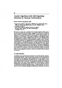
Fig. 1.

100

200

300

400 Generations

500

600

700

800

Development of K for GAHSAT (top) and GASAT (bottom).

to GAHSAT show the same effect, but even stronger. The reason for this algorithm behavior can be found in the curves of Figure 1 that exhibit the development of K during a run. As shown in those plots the selection pressure is increasing (until approximately generation 300). In the large, this implies that formula 4 results in increasing K. However, while it is theoretically possible (and numerically reasonable to assume) that K would continue to grow, Figure 1 shows that this does not happen, but for GASAT it stabilizes at K = 2.

As for the research questions from the introduction, we have demonstrated that self-adapting a global parameter, like the tournament size K, is possible and can lead to better GA performance. This is a new result. Regarding the second research question, we found that regulating K by pure inheritance is not as powerful as regulating it by a heuristic and inheritance. This work is being followed up by applying the idea of aggregating local votes for other global parameters, like population size. Furthermore, we are to make a broad comparative study on the effect of the present parameter update mechanism (formula 2) on other parameters.

1588

2 that

was, nota bene, introduced for mutation parameters

R EFERENCES [1] E.H.L. Aarts and J. Korst. Simulated Annealing and Boltzmann Machines. Wiley, Chichester, UK, 1989. [2] T. B¨ack, A.E. Eiben, and N.A.L. van der Vaart. An empirical study on GAs ”without parameters”. In M. Schoenauer, K. Deb, G. Rudolph, X. Yao, E. Lutton, J.J. Merelo, and H.-P. Schwefel, editors, Proceedings of the 6th Conference on Parallel Problem Solving from Nature, number 1917 in Lecture Notes in Computer Science, pages 315–324. Springer, Berlin, 2000. [3] T. B¨ack, D.B. Fogel, and Z. Michalewicz, editors. Evolutionary Computation 1: Basic Algorithms and Operators. Institute of Physics Publishing, Bristol, 2000. [4] Th. B¨ack and M. Sch¨utz. Intelligent mutation rate control in canonical genetic algorithms. In Zbigniew W. Ras and Maciej Michalewicz, editors, Foundations of Intelligent Systems, 9th International Symposium, ISMIS ’96, Zakopane, Poland, June 9-13, 1996, Proceedings, volume 1079 of Lecture Notes in Computer Science, pages 158–167. Springer, Berlin, Heidelberg, New York, 1996. [5] A. Dukkipati, N. M. Musti, and S. Bhatnagar. Cauchy annealing schedule: An annealing schedule for boltzmann selection scheme in evolutionary algorithms. pages 55–62. [6] A.E. Eiben, R. Hinterding, and Z. Michalewicz. Parameter control in evolutionary algorithms. IEEE Transactions on Evolutionary Computation, 3(2):124–141, 1999. [7] A.E. Eiben, E. Marchiori, and V.A. Valko. Evolutionary Algorithms with on-the-fly Population Size Adjustment. In X. Yao et al., editor, Parallel Problem Solving from Nature, PPSN VIII, number 3242 in Lecture Notes in Computer Science, pages 41–50. Springer, Berlin, Heidelberg, New York, 2004. [8] A.E. Eiben and J.E. Smith. Introduction to Evolutionary Computing. Springer, 2003. [9] D.B. Fogel. Other selection methods. In B¨ack et al. [3], chapter 27, pages 201–204. [10] L. Gonzalez and J. Cannady. A self-adaptive negative selection approach for anomaly detection. In 2004 Congress on Evolutionary Computation (CEC’2004), pages 1561–1568. IEEE Press, Piscataway, NJ, 2004. [11] P.J.B. Hancock. A comparison os selection mechanisms. In B¨ack et al. [3], chapter 29, pages 212–227. [12] N. Hansen, A. Gawelczyk, and A. Ostermeier. Sizing the population with respect to the local progress in (1, lambda)-evolution strategies. In Proceedings of the IEEE Conference on Evolutionary Computation, pages 80–85. IEEE Press, 1995. (Authors in alphabetical order). [13] G. Hardin. The tradegy of the commons. Science, 162:1243–1248, December 1968. [14] M. Herdy. The number of offspring as a strategy parameters in hierarchically organized evolution strategies. ACM SIGBIO Newsletter, 13(2):2–9, 1993. [15] S.W. Mahfoud. Boltzmann selection. In B¨ack et al. [3], chapter 26, pages 195–200. [16] E. Poupaert and Y. Deville. Acceptance driven local search and evolutionary algorithms. In L. Spector, E. Goodman, A. Wu, W.B. Langdon, H.-M. Voigt, M. Gen, S. Sen, M. Dorigo, S. Pezeshk, M. Garzon, and E. Burke, editors, Proceedings of the Genetic and Evolutionary Computation Conference (GECCO-2001), pages 1173– 1180. Morgan Kaufmann, 2001. [17] W.M. Spears. Evolutionary Algorithms: the role of mutation and recombination. Springer, Berlin, Heidelberg, New York, 2000. [18] E. Zitzler and S. K¨unzli. Indicator-based selection in multiobjective search. In E.K. Burke X. Yao, J.A. Lozano, J. Smith, J.J.M. Guervos, J.A. Bullinaria, J.E. Rowe, P. Tino, A. Kaban, and H.-P. Schwefel, editors, PPSN, number 3242 in Lecture Notes in Computer Science, pages 832–842. Springer, Berlin, Heidelberg, New York, 2004.

1

0.9

0.8

0.7

0.6

0.5

0.4

0.3 Best Fitness Mean Fitness Worst Fitness Diversity

0.2

0.1

0

100

200

300

400 Generations

500

600

700

800

1

0.9

0.8

0.7

0.6

0.5

0.4

0.3

0.2 Best Fitness Mean Fitness Worst Fitness Diversity

0.1

0

0

100

200

300

400 Generations

500

600

700

800

1

0.9

0.8

0.7

0.6

0.5

0.4

0.3

0.2 Best Fitness Mean Fitness Worst Fitness Diversity

0.1

0

0

100

200

300

400 Generations

500

600

700

800

Fig. 2. A successful run with 10 peaks of SGA (top), GAHSAT (middle) and GASAT (bottom).

1589